


Introduction
Mathematical optimization is the minimization (or maximization) of a function under given constraint conditions. Such mathematical optimization problems appear in various fields such as economics and physics, and many machine learning algorithms reduce to mathematical optimization problems. Therefore, knowing mathematical optimization and its solution methods should help in understanding the fundamental parts of machine learning.
In this article, I will explain the “Method of Lagrange Multipliers,” a powerful technique when solving mathematical optimization problems.
Minimizing a function under constraint conditions can be expressed as follows:
\begin{align*}
\min_{\bm{x}}\ &f(\bm{x}), \\
{\rm subject\ to\ }\ &g(\bm{x}) = 0.
\end{align*}
First, let’s try to solve a mathematical optimization problem straightforwardly without using the method of Lagrange multipliers.
As an example, consider:
\begin{align*}
\min_{x,y}\ &xy, \\
{\rm subject\ to\ }\ &x – y + 4 = 0.
\end{align*}
“Find the minimum value of $xy$ when real numbers $x, y$ satisfy $x – y + 4 = 0$.”
From the constraint condition, $y = x + 4$, so
\begin{align*}
xy &= x (x + 4) \\
&= x^2 + 4x \\
&= (x + 2)^2 – 4.
\end{align*}
Therefore, the minimum value is $-4$ when $x=-2$.
If the number of variables is small and the problem is simple like this, it can be solved easily.
However, what about the following problem?
\max_{n_1, \dots, n_m}\ &\frac{N!}{\displaystyle{\prod_{i=1}^m(n_i !)}}, \\
{\rm subject\ to\ }\ &\sum_{i=1}^m n_i \varepsilon_i = E,\ \sum_{i=1}^m n_i = N. \end{align*}
Or, what about the following problem?
\min_{w_1, \dots, w_n}\ &\frac{1}{2}\sqrt{w_1^2 + \cdots + w_n^2}, \\
{\rm subject\ to\ }\ &y^{(i)}\left(\sum_{j=1}^n w_j x_j^{(i)} + b\right) \geq 1, \ \ \ i = 1, 2, \cdots, n.\end{align*}
The problems are too complex, and it seems difficult to solve them as we did before.
(Incidentally, the former is a problem that gives the Boltzmann distribution, which is important in physics, and the latter is a problem that gives the machine learning algorithm called Support Vector Machine)
\begin{align*}
\newcommand{\d}{\mathrm{d}}
\newcommand{\pd}{\partial}
\end{align*}
If it is an unconstrained problem, the stationary points (points where the derivative of the function becomes 0) can be found by solving the system of equations where the gradient vector of the objective function $f(\bm{x})$ is the zero vector: $\nabla_{\! \bm{x}}\,f(\bm{x}) = \bm{0}$. If $f(\bm{x})$ is a convex function, that point becomes the minimum value (or maximum value).
Does such a solution method like the unconstrained case exist even for constrained problems? If so, we could easily find solutions even for complex problems like those above. …Such a solution method exists! It is what is called the “Method of Lagrange Multipliers.”
Method of Lagrange Multipliers (Equality Constraints)
The method of Lagrange multipliers is a method for finding the stationary points of a multivariate function under constraints between variables. Using this, the optimization problem
\begin{align*}
\min_{\bm{x}}\ &f(\bm{x}), \\
{\rm subject\ to\ }\ &g(\bm{x}) = 0
\end{align*} can be found as follows.
(Hereafter, we assume the function being considered is a downward convex function.)
Define a real-valued function called the Lagrangian function as
\begin{align*}
L(\bm{x}, \lambda) = f(\bm{x}) – \lambda g(\bm{x})
\end{align*}.
At this time, the problem of finding the extremum of $f(\bm{x})$ under the constraint condition $g(\bm{x}) = 0$ can be reduced to the problem of finding the solution to the following system of equations.
\begin{align*}
&\nabla_{\! \bm{x}}\, L(\bm{x}, \lambda) = \bm{0}, \\
\\
&\frac{\pd L(\bm{x}, \lambda)}{\pd \lambda} = 0.
\end{align*}
In the method of Lagrange multipliers, by considering the Lagrangian function $L(\bm{x}, \lambda)$ which fuses the objective function $f(\bm{x})$ and the constraint equation $g(\bm{x})$, we can solve the constrained problem as a standard extremum problem. Here, the coefficient $\lambda$ of the constraint equation is called the Lagrange multiplier.
As an example, let’s solve the problem at the beginning using the method of Lagrange multipliers.
“Find the minimum value of $xy$ when real numbers $x, y$ satisfy $x\, – y + 4 = 0$.”
Let $f(x, y) = xy,\ g(x, y) = x\, – y + 4$.
Defining the Lagrangian function $L$ as
\begin{align*}
L(x, y, \lambda) &= f(x,y)\, – \lambda g(x,y) \\
&= xy\, – \lambda(x – y + 4)
\end{align*}
, from the method of Lagrange multipliers, $x, y$ satisfying the following system of equations become the extrema.
\begin{align*}
\frac{\pd L}{\pd x} &= y\, – \lambda = 0 \\
\frac{\pd L}{\pd y} &= x + \lambda = 0 \\
\frac{\pd L}{\pd \lambda} &= -x + y -4 = 0
\end{align*}
Solving the above system of equations, we obtain $x = -2, y = 2, \lambda = 2$.
Therefore, the minimum value is $-4$.
Also, in machine learning algorithms, the method of Lagrange multipliers appears in the theory of Principal Component Analysis (PCA).
Why does it hold?
Why does it hold? Leaving rigor aside, we will consider the geometric interpretation in the case of a function of two variables.
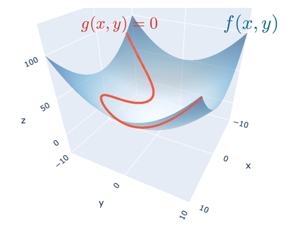
We illustrate the objective function $f(x, y)$ and the constraint function $g(x, y) = 0$. The two-variable function $f(x, y)$ is drawn as a curved surface, and $g(x, y) = 0$ as a curve.
Finding the minimum value of the objective function under the constraint condition means finding the position with the lowest elevation of the objective function: $f(x, y)$ on this curve: $g(x, y) = 0$.
Let’s assume this curve is a mountain path. When you are at the lowest elevation along the path, you must be walking along a contour line. Why? Because if you were going up or down the mountain path, you would be crossing contour lines as you proceed. The moment when the elevation is lowest along the path is exactly when you are not crossing contour lines, that is, the position where you are walking along a contour line. Geometrically, this can be regarded as the situation where the tangent to the curve and the tangent to the contour line overlap.
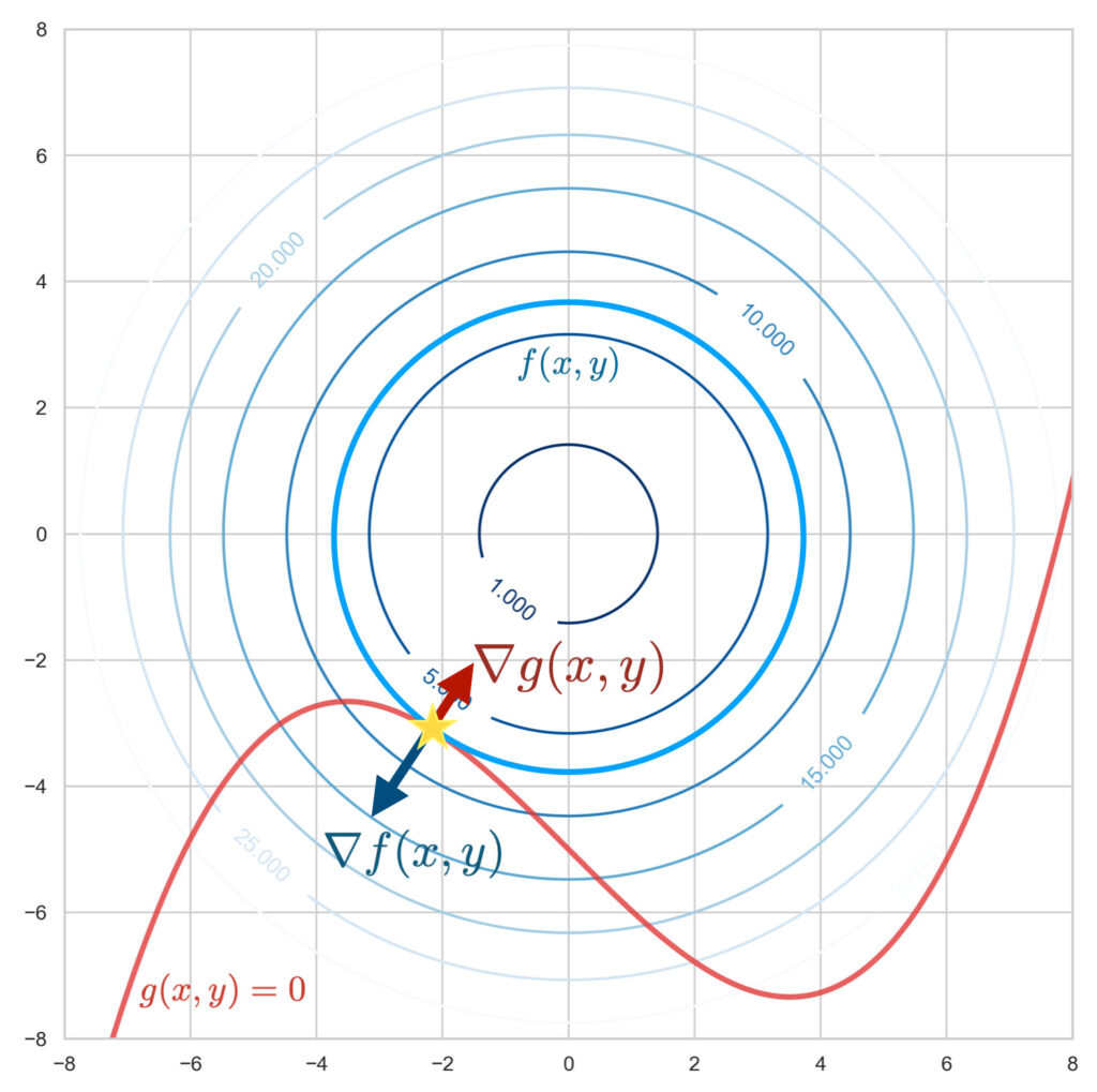
To find the point where these two tangent lines overlap (the star mark in the figure above), it is good to use the gradients of the functions. The gradient vectors $\nabla_{\! x, y}\, f(x, y),\ \nabla_{\! x, y}\, g(x, y)$ represent vectors perpendicular to the contour lines and perpendicular to the curve, respectively.
The place where the gradient of $f(x, y)$, $\nabla_{\! x, y}\, f(x,y)$, and the gradient of $g(x, y)$, $\nabla_{\! x, y}\, g(x,y)$, are parallel is the point where the two tangent lines overlap, that is, the position where the objective function is minimized under the constraint condition. This can be expressed by the following equation.
\begin{align*}
\nabla_{\! x, y}\, f(x,y) = \lambda \nabla_{\! x, y}\, g(x, y)
\end{align*}Here, $\lambda$ is a variable that appears because it is sufficient for the gradient directions of $f$ and $g$ to match, and their lengths do not matter; it is called the “Lagrange multiplier.”
Transforming the above equation,
\begin{align*}
\nabla_{\! x, y}\, \left\{f(x,y) – \lambda g(x, y) \right\} = 0
\end{align*}Using the Lagrangian function: $L(x, y) \equiv f(x, y) – \lambda g(x, y)$, it can be rewritten as
\begin{align*}
\nabla_{\! x,y}\, L(x, y) = 0
\end{align*}.
On the other hand, the constraint condition $g(x, y) = 0$ can be expressed as $\frac{\pd L}{\pd \lambda} = 0$.
In this way, by the method of Lagrange multipliers, constrained problems can be solved as standard extremum problems.