


Introduction
In the previous article, we discussed the theory of Hard Margin SVM.
Based on that, this time we will implement it using Python.

Also, the following code runs on Google Colab.

\begin{align*}
\newcommand{\mat}[1]{\begin{pmatrix} #1 \end{pmatrix}}
\newcommand{\f}[2]{\frac{#1}{#2}}
\newcommand{\pd}[2]{\frac{\partial #1}{\partial #2}}
\newcommand{\d}[2]{\frac{{\rm d}#1}{{\rm d}#2}}
\newcommand{\T}{\mathsf{T}}
\newcommand{\(}{\left(}
\newcommand{\)}{\right)}
\newcommand{\{}{\left\{}
\newcommand{\}}{\right\}}
\newcommand{\[}{\left[}
\newcommand{\]}{\right]}
\newcommand{\dis}{\displaystyle}
\newcommand{\eq}[1]{{\rm Eq}(\ref{#1})}
\newcommand{\n}{\notag\\}
\newcommand{\t}{\ \ \ \ }
\newcommand{\tt}{\t\t\t\t}
\newcommand{\argmax}{\mathop{\rm arg\, max}\limits}
\newcommand{\argmin}{\mathop{\rm arg\, min}\limits}
\def\l<#1>{\left\langle #1 \right\rangle}
\def\us#1_#2{\underset{#2}{#1}}
\def\os#1^#2{\overset{#2}{#1}}
\newcommand{\case}[1]{\{ \begin{array}{ll} #1 \end{array} \right.}
\newcommand{\s}[1]{{\scriptstyle #1}}
\definecolor{myblack}{rgb}{0.27,0.27,0.27}
\definecolor{myred}{rgb}{0.78,0.24,0.18}
\definecolor{myblue}{rgb}{0.0,0.443,0.737}
\definecolor{myyellow}{rgb}{1.0,0.82,0.165}
\definecolor{mygreen}{rgb}{0.24,0.47,0.44}
\newcommand{\c}[2]{\textcolor{#1}{#2}}
\newcommand{\ub}[2]{\underbrace{#1}_{#2}}
\end{align*}
Hard Margin SVM Theory Overview
Let $X$ denote the observed $n$ $p$-dimensional data points, and $\bm{y}$ denote the set of $n$ label variables, expressed as follows:
\us X_{[n \times p]} = \mat{x_1^{(1)} & x_2^{(1)} & \cdots & x_p^{(1)} \\
x_1^{(2)} & x_2^{(2)} & \cdots & x_p^{(2)} \\
\vdots & \vdots & \ddots & \vdots \\
x_1^{(n)} & x_2^{(2)} & \cdots & x_p^{(n)}}
=
\mat{ – & \bm{x}^{(1)\T} & – \\
– & \bm{x}^{(2)\T} & – \\
& \vdots & \\
– & \bm{x}^{(n)\T} & – \\},
\t
\us \bm{y}_{[n \times 1]} = \mat{y^{(1)} \\ y^{(2)} \\ \vdots \\ y^{(n)}}.
\end{align*}
From the previous conclusion, the parameters determining the separating hyperplane could be calculated by the following equations:
\hat{\bm{w}} &= \sum_{\bm{x}^{(i)} \in S} \hat{\alpha}_i y^{(i)} \bm{x}^{(i)}, \\
\hat{b} &= \f{1}{|S|} \sum_{\bm{x}^{(i)} \in S} (y^{(i)} – \hat{\bm{w}}^\T \bm{x}^{(i)}).
\end{align}
(Here, $S$ is the set of support vectors)
Also, $\bm{\alpha} = (\alpha_1, \alpha_2, \dots, \alpha_n)^\T$ is the set of Lagrange multipliers, and here we find its optimal solution $\hat{\bm{\alpha}}$ using the gradient descent method.
\bm{\alpha}^{[t+1]} = \bm{\alpha}^{[t]} + \eta \pd{\tilde{L}(\bm{\alpha})}{\bm{\alpha}}.
\end{align*}
The value of the gradient vector $\pd{\tilde{L}(\bm{\alpha})}{\bm{\alpha}}$ was calculated as
\us H_{[n \times n]} \equiv \us \bm{y}_{[n \times 1]} \us \bm{y}^{\T}_{[1 \times n]} \odot \us X_{[n \times p]} \us X^{\T}_{[p \times n]}
\end{align}
using
\begin{align}
\pd{\tilde{L}(\bm{\alpha})}{\bm{\alpha}} = \bm{1}\, – H \bm{\alpha}.
\end{align}
.
Implementing Hard Margin SVM from Scratch
Based on the above, we will implement the Hard Margin SVM from scratch.
import numpy as np

class HardMarginSVM:
    """
    Attributes
    ----------
    eta : float
        Learning rate
    epoch : int
        Number of epochs
    random_state : int
        Random seed
    is_trained : bool
        Training completion flag
    num_samples : int
        Number of training samples
    num_features : int
        Number of features
    w : NDArray[float]
        Parameter vector: ndarray of shape (num_features, )
    b : float
        Intercept parameter
    alpha : NDArray[float]
        Lagrange multipliers: ndarray of shape (num_samples, )

    Methods
    -------
    fit -> None
        Fit the parameter vector to the training data
    predict -> NDArray[int]
        Return predicted values
    """
    def __init__(self, eta=0.001, epoch=1000, random_state=42):
        self.eta = eta
        self.epoch = epoch
        self.random_state = random_state
        self.is_trained = False

    def fit(self, X, y):
        """
        Fit the parameter vector to the training data

        Parameters
        ----------
        X : NDArray[NDArray[float]]
            Training data: matrix of shape (num_samples, num_features)
        y : NDArray[float]
            Training data labels: ndarray of shape (num_samples)
        """
        self.num_samples = X.shape[0]
        self.num_features = X.shape[1]
        # Initialize parameter vector with zeros
        self.w = np.zeros(self.num_features)
        self.b = 0
        # Random number generator
        rgen = np.random.RandomState(self.random_state)
        # Initialize alpha (Lagrange multipliers) using normal random numbers
        self.alpha = rgen.normal(loc=0.0, scale=0.01, size=self.num_samples)
        # Solve the dual problem using gradient descent
        for _ in range(self.epoch):
            self._cycle(X, y)

        # Get indices of support vectors
        indexes_sv = [i for i in range(self.num_samples) if self.alpha[i] != 0]
        # Calculate w (Eq. 1)
        for i in indexes_sv:
            self.w += self.alpha[i] * y[i] * X[i]
        # Calculate b (Eq. 2)
        for i in indexes_sv:
            self.b += y[i] - (self.w @ X[i])
        self.b /= len(indexes_sv)
        # Set training completion flag
        self.is_trained = True

    def predict(self, X):
        """
        Return predicted values

        Parameters
        ----------
        X : NDArray[NDArray[float]]
            Data to classify: matrix of shape (any, num_features)
        Returns
        -------
        result : NDArray[int]
            Classification result -1 or 1: ndarray of shape (any, )
        """
        if not self.is_trained:
            raise Exception('This model is not trained.')

        hyperplane = X @ self.w + self.b
        result = np.where(hyperplane > 0, 1, -1)
        return result

    def _cycle(self, X, y):
        """
        One cycle of gradient descent

        Parameters
        ----------
        X : NDArray[NDArray[float]]
            Training data: matrix of shape (num_samples, num_features)
        y : NDArray[float]
            Training data labels: ndarray of shape (num_samples)
        """
        y = y.reshape([-1, 1])  # Reshape to (num_samples, 1) matrix
        H = (y @ y.T) * (X @ X.T)  # (Eq. 3)
        # Calculate gradient vector
        grad = np.ones(self.num_samples) - H @ self.alpha  # (Eq. 4)
        # Update alpha (Lagrange multipliers)
        self.alpha += self.eta * grad
        # Each component of alpha must be non-negative, so set negative components to zero
self.alpha = np.where(self.alpha < 0, 0, self.alpha)Verifying SVM Operation using the Iris Dataset
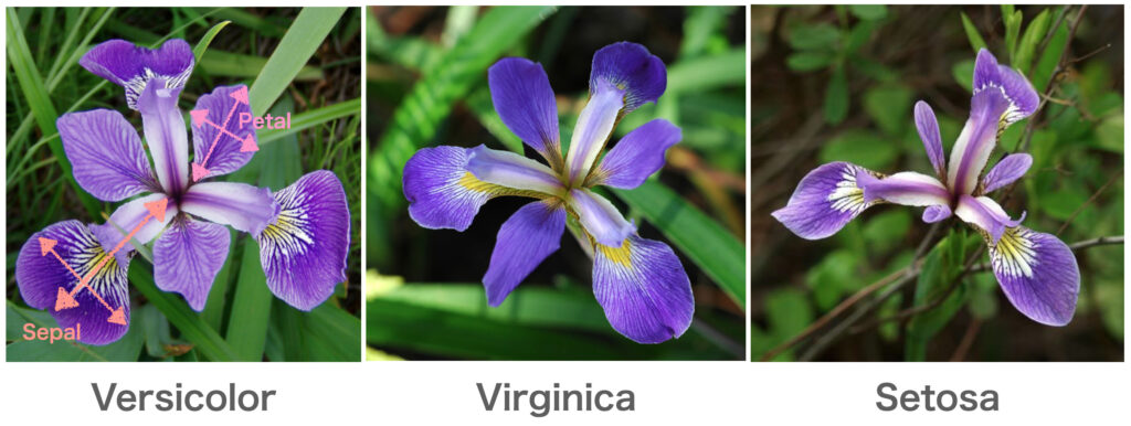
We will use the iris dataset as an example. The iris dataset consists of the petal and sepal lengths of three varieties: Versicolour, Virginica, and Setosa.
Let’s load the iris dataset using the scikit-learn library.
import pandas as pd
from sklearn.datasets import load_iris

iris = load_iris()  # Load iris dataset
df_iris = pd.DataFrame(iris.data, columns=iris.feature_names)
df_iris['class'] = iris.target
df_iris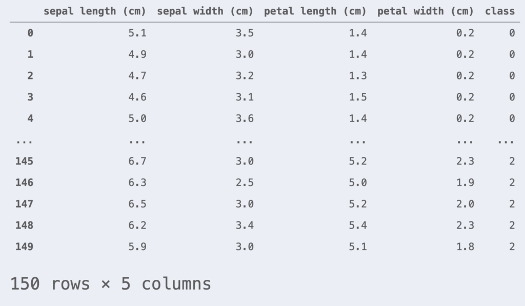
This time, we will perform binary classification. We will focus only on data with class = 0, 1. Also, for simplicity, we will use two features: petal length and petal width.
df_iris = df_iris[df_iris['class'] != 2]  # Get only data with class = 0, 1
df_iris = df_iris[['petal length (cm)', 'petal width (cm)', 'class']]
X = df_iris.iloc[:, :-1].values
y = df_iris.iloc[:, -1].values
y = np.where(y==0, -1, 1) # Change label of class = 0 to -1Also, we perform standardization so that the dataset has a mean of 0 and a standard deviation of 1.
from sklearn.preprocessing import StandardScaler

# Create standardization instance (convert to mean=0, std=1)
sc = StandardScaler()
X_std = sc.fit_transform(X)To evaluate the generalization performance of the model, we split the dataset into a training dataset and a test dataset. Here, we split it at a ratio of 80% training data and 20% test data.
from sklearn.model_selection import train_test_split

X_train, X_test, y_train, y_test = train_test_split(X_std, y, test_size=0.2, random_state=42, stratify=y)We also define a plotting class here.
# Define classification boundary plotting class
import matplotlib.pyplot as plt
from matplotlib.colors import ListedColormap

class DecisionPlotter:
    def __init__(self, X, y, classifier, test_idx=None):
        self.X = X
        self.y = y
        self.classifier = classifier
        self.test_idx = test_idx
        self.colors = ['#de3838', '#007bc3', '#ffd12a']
        self.markers = ['o', 'x', ',']
        self.labels = ['setosa', 'versicolor', 'virginica']

    def plot(self):
        cmap = ListedColormap(self.colors[:len(np.unique(self.y))])
        # Generate grid points
        xx1, xx2 = np.meshgrid(
            np.arange(self.X[:,0].min()-1, self.X[:,0].max()+1, 0.01),
            np.arange(self.X[:,1].min()-1, self.X[:,1].max()+1, 0.01))
        # Get predicted values for each meshgrid
        Z = self.classifier.predict(np.array([xx1.ravel(), xx2.ravel()]).T)
        Z = Z.reshape(xx1.shape)
        # Plot contours
        plt.contourf(xx1, xx2, Z, alpha=0.2, cmap=cmap)
        plt.xlim(xx1.min(), xx1.max())
        plt.ylim(xx2.min(), xx2.max())
        # Plot data points for each class
        for idx, cl, in enumerate(np.unique(self.y)):
            plt.scatter(
                x=self.X[self.y==cl, 0], y=self.X[self.y==cl, 1],
                alpha=0.8,
                c=self.colors[idx],
                marker=self.markers[idx],
                label=self.labels[idx])
        # Highlight test data
        if self.test_idx is not None:
            X_test, y_test = self.X[self.test_idx, :], self.y[self.test_idx]
            plt.scatter(
                X_test[:, 0], X_test[:, 1],
                alpha=0.9,
                c='None',
                edgecolor='gray',
                marker='o',
                s=100,
                label='test set')
plt.legend()Now, let’s verify the operation of the SVM using the iris dataset.
# Train SVM parameters
hard_margin_svm = HardMarginSVM()
hard_margin_svm.fit(X_train, y_train)

# Combine training and test data
X_comb = np.vstack((X_train, X_test))
y_comb = np.hstack((y_train, y_test))

# Plot
dp = DecisionPlotter(X=X_comb, y=y_comb, classifier=hard_margin_svm, test_idx=range(len(y_train), len(y_comb)))
dp.plot()
plt.xlabel('petal length [standardized]')
plt.ylabel('petal width [standardized]')
plt.show()
We were able to plot the decision curve in this way.
Implementation of SVM using scikit-learn
Execution of SVM using scikit-learn can be done as follows.
from sklearn import svm

sk_svm = svm.LinearSVC(C=1e10, random_state=42)
sk_svm.fit(X_train, y_train)
# Combine training and test data
X_comb = np.vstack((X_train, X_test))
y_comb = np.hstack((y_train, y_test))

# Plot
dp = DecisionPlotter(X=X_comb, y=y_comb, classifier=sk_svm, test_idx=range(len(y_train), len(y_comb)))
dp.plot()
plt.xlabel('petal length [standardized]')
plt.ylabel('petal width [standardized]')
plt.show()
We were also able to plot the decision curve using scikit-learn in this way.
The above code can be tested here ▼
▼ Implementation of Soft Margin SVM is here