Understanding Taylor Expansion Theory: Why Can Functions Be Expressed as Polynomials?

Table of Contents

Introduction
Why Can It Be Expressed as a Polynomial?
Finding the Values of the Coefficients

Introduction

I believe the beauty of Taylor expansion lies in the fact that functions can be expressed as polynomials.

When I first learned about it, I was fascinated by why a certain function \(f(x)\) could be represented as a polynomial. This time, I’d like to understand the reason in a relaxed manner.

Taylor expansion is expressed as follows.

Taylor Expansion

When a function \(f(x)\) is infinitely differentiable in an interval containing \(x = a\), \(f(x)\) is

\begin{eqnarray*}
f(x) &=& f(a) + f^{\prime}(a)\, (x\, – a) + \frac{1}{2!}f^{\prime\prime}(a)\, (x-a)^2 + \cdots + \frac{1}{n!}f^{(n)}(a)\, (x-a)^n + \cdots \\
&=& \sum_{k = 0}^{\infty} \frac{1}{k!}f^{(k)}(a)\, (x-a)^k
\end{eqnarray*}

and this is called the “Taylor expansion around \(a\)”.

Or,

Taylor Expansion

\begin{eqnarray*}
f(x + a) &=& f(x) + f^{\prime}(x)\, a + \frac{1}{2!}f^{\prime\prime}(x)\, a^2 + \cdots + \frac{1}{n!}f^{(n)}(x)\, a^n + \cdots \\
&=& \sum_{k = 0}^{\infty} \frac{1}{k!}f^{(k)}(x)\, a^k
\end{eqnarray*}

it may also be expressed in this form. Here, let’s derive the first expression.

Why Can It Be Expressed as a Polynomial?

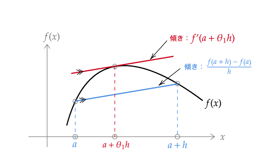
Let’s suppose that the function \(f(x)\) has the shape shown in the figure above.

Suddenly, let’s consider a straight line passing through the point \( (a,\, f(a)) \) and the point \( (a + h,\, f(a + h)) \) (the blue line in Figure 1). The slope of this line is

\begin{eqnarray}
\frac{f(a + h)\, – f(a)}{h}\tag{1}
\end{eqnarray}

Here, there exists somewhere between \(a\) and \(a + h\) a value of \(x\) for which the slope of the tangent line \(f^{\prime}(x)\) of the function \(f(x)\) is exactly equal to (1) (mean value theorem). So if we denote that value of \(x\) as \(a + \theta_1 h\ (0 < \theta_1 < 1)\), then

\begin{eqnarray*}
f^{\prime}(a + \theta_1 h) = \frac{f(a + h)\, – f(a)}{h}
\end{eqnarray*}

holds. Rearranging,

\begin{eqnarray}
f(a + h) = f(a) + f^{\prime}(a + \theta_1 h)\, h \tag{2}
\end{eqnarray}

However, since our goal is to represent the function \(f\) as a polynomial, we want to do something about \(f^{\prime}(a + \theta_1 h) \) in the above equation.

So next, let’s consider the graph of the function \(f^{\prime}(x)\). Suppose it has the shape shown in the figure below.

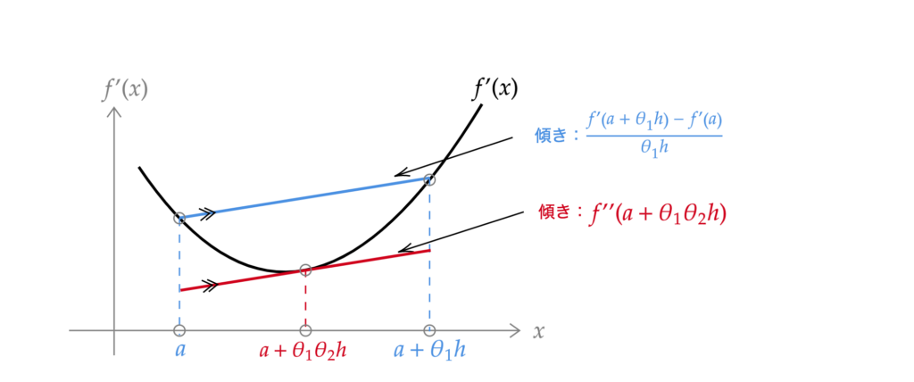
Similarly to before, let’s consider a straight line passing through the point \( (a,\, f^{\prime}(a)) \) and the point \( (a + \theta_1 h,\, f^{\prime}(a +\theta_1 h)) \) (the blue line in Figure 2). The slope of this line is

\begin{eqnarray*}
\frac{f^{\prime}(a + \theta_1 h)\, – f^{\prime}(a)}{\theta_1 h}\tag{3}
\end{eqnarray*}

Here, there exists somewhere between \(a\) and \(a + \theta_1 h\) a value of \(x\) for which the slope of the tangent line \(f^{\prime\prime}(x)\) of the function \(f^{\prime}(x)\) is exactly equal to (3). So if we denote that value of \(x\) as \(a + \theta_1 \theta_2 h\ (0 < \theta_2 < 1)\), then

\begin{eqnarray*}
f^{\prime\prime}(a + \theta_1 \theta_2 h) = \frac{f^{\prime}(a + h)\, – f^{\prime}(a)}{\theta_1 h}
\end{eqnarray*}

holds. Rearranging,

\begin{eqnarray*}
f^{\prime}(a + h) = f^{\prime}(a) + \theta_1 f^{\prime\prime}(a + \theta_1 \theta_2 h)\, h
\end{eqnarray*}

Substituting this equation into (2),

\begin{eqnarray*}
f(a + h) = f(a) + f^{\prime}(a)\, h + \theta_1 f^{\prime\prime}(a + \theta_1 \theta_2 h)\, h^2
\end{eqnarray*}

By repeating such operations many times, it seems that the function \(f\) can be expressed as a polynomial in \(h\). If the function \(f(x) \) is infinitely differentiable around \(a\), then

\begin{eqnarray*}
f(a + h) &=& f(a) + f^{\prime}(a)\, h + \theta_1 f^{\prime\prime}(a)\, h^2 + \theta_1 \theta_2 f^{(3)}(a + \theta_1 \theta_2 \theta_3 h)\, h^3 \\
\\
f(a + h) &=& f(a) + f^{\prime}(a)\, h + \theta_1 f^{\prime\prime}(a)\, h^2 + \theta_1 \theta_2 f^{(3)}(a)\, h^3 + \theta_1 \theta_2 \theta_3 f^{(4)}(a + \theta_1 \theta_2 \theta_3 \theta_4 h)\, h^4 \\
\\
&\vdots & \\
\\
f(a + h) &=& f(a) + f^{\prime}(a)\, h + \theta_1 f^{\prime\prime}(a)\, h^2 + \theta_1 \theta_2 f^{(3)}(a)\, h^3 + \cdots + \theta_1 \theta_2 \cdots \theta_{n-1} f^{(n)}(a)\, h^n + \cdots
\end{eqnarray*}

Rewriting the coefficient of each term \(\theta_1 \theta_2 \cdots \) as \(c\), and \(h = x-a\),

\begin{eqnarray*}
f(x) = f(a) + c_1f^{\prime}(a)\, (x – a) + c_2f^{\prime\prime}(a)\, (x-a)^2 &+& c_3f^{(3)}(a)\, (x-a)^3 \\ &+& \cdots + c_n f^{(n)}(a)\, (x-a)^n + \cdots \tag{☆}
\end{eqnarray*}

we were able to transform it. But what are the values of the coefficients \(c_i\)??

Finding the Values of the Coefficients

To find the values of the coefficients \(c_i\), let’s take the first derivative of equation (☆) with respect to \(x\). Then,

\begin{eqnarray*}
f^{\prime}(x) = c_1f^{\prime}(a) + 2\, c_2f^{\prime\prime}(a)\, (x-a) + 3\, c_3f^{(3)}(a)\, (x-a)^2 + \cdots + n\, c_n f^{(n)}(a)\, (x-a)^{n-1} + \cdots
\end{eqnarray*}

If we substitute \(x = a\), all terms on the right side except the first term become 0, so

\begin{eqnarray*}
f^{\prime}(a) &=& c_1 f^{\prime}(a) \\
∴ c_1 &=& 1
\end{eqnarray*}

and we have found \(c_1\).

Similarly, taking the second derivative of equation (☆) with respect to \(x\),

\begin{eqnarray*}
f^{\prime\prime}(x) = 2\cdot 1\, c_2f^{\prime\prime}(a) + 3\cdot 2\, c_3f^{(3)}(a)\, (x-a) + \cdots + n \cdot (n-1)\, c_n f^{(n)}(a)\, (x-a)^{n-2} + \cdots
\end{eqnarray*}

Substituting \(x = a\),

\begin{eqnarray*}
f^{\prime\prime}(a) &=& 2!\, c_2 f^{\prime\prime}(a) \\
∴ c_1 &=& \frac{1}{2!}
\end{eqnarray*}

Taking the third derivative of equation (☆) with respect to \(x\),

\begin{eqnarray*}
f^{(3)}(x) = 3 \cdot 2\cdot 1\, c_3f^{(3)}(a) + \cdots + n \cdot (n-1) \cdot (n-2)\, c_n f^{(n)}(a)\, (x-a)^{n-3} + \cdots
\end{eqnarray*}

Substituting \(x = a\),

\begin{eqnarray*}
f^{\prime\prime}(a) &=& 3!\, c_3 f^{\prime\prime}(a) \\
∴ c_3 &=& \frac{1}{3!}
\end{eqnarray*}

Therefore, the coefficient of the \(n\)th term \(c_n\) can be found by taking the \(n\)th derivative of equation (☆) with respect to \(x\) and substituting \(x = a\),

\begin{eqnarray*}
c_n = \frac{1}{n!}
\end{eqnarray*}

Therefore, equation (☆) becomes

\begin{eqnarray*}
f(x) = f(a) + f^{\prime}(a)\, (x – a) + \frac{1}{2!}f^{\prime\prime}(a)\, (x-a)^2 + \cdots + \frac{1}{n!}f^{(n)}(a)\, (x-a)^n + \cdots
\end{eqnarray*}

and we have successfully derived the expression for Taylor expansion.

For examples of Taylor expansion, see here▼