


Transformation of Random Variables (Monotonic Mapping Case)
Let us consider deriving the probability density function $f_Y(y)$ of $Y$ in terms of the probability density function $f_X(x)$ of $X$, when a random variable $X$ is transformed through a function $g(\cdot)$ as
\begin{eqnarray*}
Y = g(X)
\end{eqnarray*}
Let $f_X(x)$ be the probability density function of random variable $X$, and let $Y = g(X)$. When $g(x)$ is a monotonic function and $g^{-1}(y)$ is differentiable, the probability density function of $Y$ is given by:
f_Y(y) = f_X\left(g^{-1}(y) \right) \left| \frac{\mathrm{d}}{\mathrm{d}y}g^{-1}(y) \right|
\end{eqnarray*}
First, let us consider this through a concrete example. Below, we denote the cumulative distribution function of $X$ as $F_X(x)$.
Example 1
For $Y = g(X)$, consider the case when $g(X) = a + b X$. That is, $Y = a + bX$. Here, $a, b$ are constants with $b \neq 0$. Express $f_Y$ in terms of $f_X$.
\begin{eqnarray*}
\definecolor{myblack}{rgb}{0.27,0.27,0.27}
\definecolor{myred}{rgb}{0.78,0.24,0.18}
\definecolor{myblue}{rgb}{0.0,0.443,0.737}
\definecolor{myyellow}{rgb}{1.0,0.82,0.165}
\definecolor{mygreen}{rgb}{0.24,0.47,0.44}
\end{eqnarray*}
(i) When $b > 0$
F_Y(y) = P(Y \leq y) &=& P(a + bX \leq y) \\
&=& P\left(X \leq \frac{y\,- a}{b}\right) \\
&=& F_X\left(\frac{y-a}{b}\right)
\end{eqnarray*}
Therefore,
f_Y(y) = \frac{\mathrm{d}}{\mathrm{d}y}F_Y(y) &=& \frac{\mathrm{d}}{\mathrm{d}y}F_X\left(\frac{y-a}{b}\right) \\
&=& \frac{\mathrm{d}}{\mathrm{d}x}F_X\left(\frac{y-a}{b}\right) \cdot \frac{\mathrm{d}x}{\mathrm{d}y} \\
&=& \frac{\mathrm{d}}{\mathrm{d}x}F_X\left(\frac{y-a}{b}\right) \cdot \frac{\mathrm{d}}{\mathrm{d}y} \frac{y\,- a}{b}\\
&=& f_X\left(\frac{y-a}{b}\right) \cdot \frac{1}{b}
\end{eqnarray*}
(ii) When $b < 0$
F_Y(y) = P(Y \leq y) &=& P(a + bX \leq y) \\
&=& P\left(X \textcolor{myred}{\geq} \frac{y\,- a}{b}\right) \\
&=& 1\, – P\left(X \leq \frac{y\,- a}{b}\right) \\
&=& 1- F_X\left(\frac{y-a}{b}\right)
\end{eqnarray*}
Therefore,
f_Y(y) = \frac{\mathrm{d}}{\mathrm{d}y}F_Y(y) &=& \frac{\mathrm{d}}{\mathrm{d}y}\left[ 1 \,- F_X\left(\frac{y-a}{b}\right) \right]\\
&=& – \frac{\mathrm{d}}{\mathrm{d}y} F_X\left(\frac{y-a}{b}\right) \\
&\vdots&\\
&=& – f_X\left(\frac{y-a}{b}\right) \cdot \frac{1}{b}
\end{eqnarray*}
From the above,
f_Y(y) = f_X\left(\frac{y-a}{b}\right) \cdot \frac{1}{|b|}
\end{eqnarray*}
In Example 1, you can see that $f_Y(y)$ is in the form of Theorem 1.
Now let us prove Theorem 1. For $Y = g(X)$,
(i) When $g(x)$ is a monotonically increasing function
F_{Y}(y)=P(Y \leq y) &=& P(g(X) \leq y)\\
&=&P\left(X \leq g^{-1}(y)\right) \\
&=& F_{X}\left(g^{-1}(y)\right)
\end{eqnarray*}
Therefore,
f_{Y}(y)=\frac{\mathrm{d}}{\mathrm{d} y} F_{Y}(y) &=& \frac{\mathrm{d}}{\mathrm{d} y} F_{X}\left(g^{-1}(y)\right) \\
&=&\frac{\mathrm{d}}{\mathrm{d} x} F_{X}\left(g^{-1}(y)\right) \cdot \frac{\mathrm{d}x}{\mathrm{d}y} \\
&=& f_{X}\left(g^{-1}(y)\right) \frac{d}{d y} g^{-1}(y)\tag{1}
\end{eqnarray*}
(ii) When $g(x)$ is a monotonically decreasing function
F_{Y}(y)=P(Y \leq y)&=& P(g(X) \leq y)\\
&=&P\left(X \textcolor{myred}{\geq} g^{-1}(y)\right) \\
&=&1- P\left(X \leq g^{-1}(y)\right)\\
&=&1- F_{X}\left(g^{-1}(y)\right)
\end{eqnarray*}
Therefore,
f_{Y}(y)=\frac{\mathrm{d}}{\mathrm{d} y} F_{Y}(y) &=& \frac{\mathrm{d}}{\mathrm{d} y} \left[ 1- F_{X}\left(g^{-1}(y)\right) \right]\\
&=&\textcolor{myred}{-} \frac{\mathrm{d}}{\mathrm{d} x} F_{X}\left(g^{-1}(y)\right) \cdot \frac{\mathrm{d}x}{\mathrm{d}y} \\
&=& f_{X}\left(g^{-1}(y)\right) \left( \textcolor{myred}{-} \frac{d}{d y} g^{-1}(y) \right)\tag{2}
\end{eqnarray*}
Therefore, from (1) and (2)
f_Y(y) = f_X\left(g^{-1}(y) \right) \left| \frac{\mathrm{d}}{\mathrm{d}y}g^{-1}(y) \right| \tag{☆}
\end{eqnarray*}
As an alternative expression of (☆), there is the following formula.
\begin{eqnarray*}
g\left( g^{-1}(y)\right) = y
\end{eqnarray*}
Differentiating both sides with respect to $y$,
1 &=& \frac{\mathrm{d}}{\mathrm{d}y}g\left( g^{-1}(y)\right) \\
&=& \frac{\mathrm{d}}{\mathrm{d}g^{-1}}g\left( g^{-1}(y)\right) \cdot \frac{\mathrm{d}g^{-1}}{\mathrm{d}y} \\
&=& g^{\prime}\left( g^{-1}(y)\right) \cdot \frac{\mathrm{d}g^{-1}}{\mathrm{d}y} \\
\\
&\therefore& \frac{\mathrm{d}g^{-1}}{\mathrm{d}y} = \frac{1}{g^{\prime}\left( g^{-1}(y)\right)}
\end{eqnarray*}
Substituting the above equation into (☆),
f_Y(y) = f_X\left(g^{-1}(y) \right) \left| \frac{1}{g^{\prime}\left( g^{-1}(y)\right)} \right|
\end{eqnarray*}
can also be expressed.
Transformation of Random Variables (Non-Monotonic Mapping Case)
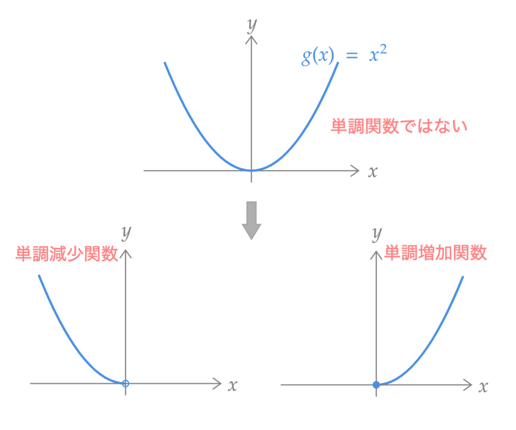
Care must be taken when $g(\cdot)$ is not a monotonic function. For example, when $Y = X^2$, it is not a monotonic function over $\mathbb{R}$. However, it is a monotonic function over $\mathbb{R}^{+}_0$ and over $\mathbb{R}^{-}$. In this way, we will consider dividing into intervals where $g(\cdot)$ becomes a monotonic function.
Example 2
For $Y = g(X)$, consider the case when $g(X) = X^2$. That is, $Y = X^2$. Express $f_Y$ in terms of $f_X$.
Let $\Omega$ be the sample space, then
F_Y(y) = P(Y \leq y) &=& P\left(X^2 \leq y \right) \\
\\
&=& P\left(X^2 \leq y\, |\, X(\omega) \geq 0,\, \omega \in \Omega \right) \\
&&\ \ + P\left(X^2 \leq y\, |\, X(\omega) < 0,\, \omega \in \Omega \right) \\
\\
&=& P\left(0 \leq X \leq \sqrt{y} \right) + P\left( -\sqrt{y} \leq X < 0 \right) \\
\\
&=& P\left(-\sqrt{y} \leq X \leq \sqrt{y} \right)\\
\\
&=& F_X(\sqrt{y} )\, – F_X(-\sqrt{y})
\end{eqnarray*}
Therefore,
f_Y(y) = \frac{\mathrm{d}}{\mathrm{d}y}F_Y(y) &=& \frac{\mathrm{d}}{\mathrm{d}y}\left[ F_X(\sqrt{y})\, – F_X(-\sqrt{y}) \right] \\
\\
&=& \frac{\mathrm{d}}{\mathrm{d}x}F_X(\sqrt{y}) \cdot \frac{\mathrm{d}}{\mathrm{d}y}\sqrt{y}\\
&&\ \ – \frac{\mathrm{d}}{\mathrm{d}x}F_X(-\sqrt{y}) \cdot \frac{\mathrm{d}}{\mathrm{d}y}( -\sqrt{y}) \\
\\
&=&\frac{1}{2 \sqrt{y}} f_{X}(\sqrt{y})+\frac{1}{2 \sqrt{y}} f_{X}(-\sqrt{y})
\end{eqnarray*}
Based on this example, let us consider the general case of $Y = g(X)$.
First, let us introduce $\mathcal{X} = \{x\ | \ f_X(x) > 0 \}$. $\mathcal{X}$ is called the support of $X$. Then the following theorem holds.
Let $f_X(x)$ be the probability density function of random variable $X$, and let $Y = g(X)$.
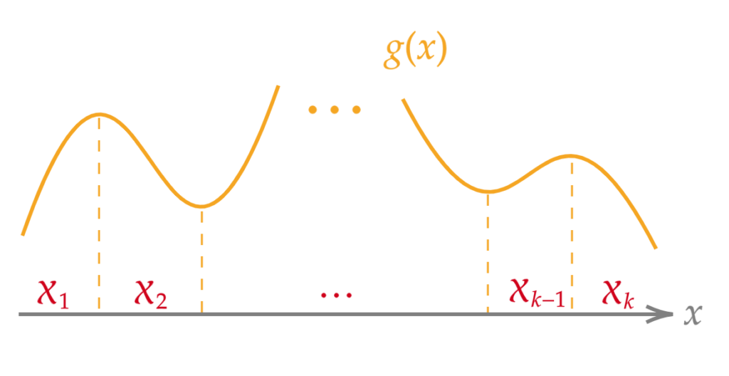
Let $\{\mathcal{X}_i\}$ be a partition of $\mathcal{X}$, and let $f_X(x)$ be continuous on each $\mathcal{X}_i\ (i= 1, \dots, k)$. When a monotonic function $g_i(x)$ defined on each $\mathcal{X}_i$ satisfies $g(x) = g_i(x)$ for $x \in \mathcal{X}_i$, and $g^{-1}_i(y)$ is differentiable, the probability density function of $Y$ is given by:
f_Y(y) = \sum_{i=1}^{k} f_{X}\left(g_{i}^{-1}(y)\right)\left|\frac{d}{d y} g_{i}^{-1}(y)\right|
\end{eqnarray*}
In essence, this means dividing into intervals where $g(x)$ becomes a monotonic function.
Finally, let us give a simple proof of Theorem 2.
F_{Y}(y)=P(Y \leq y) &=& \sum_{i=1}^{k} P\left(g(X) \leq y\ | \ X \in \mathcal{X}_{i}\right) \\
&=& \sum_{i=1}^{k} P\left(g_i(X) \leq y \right) \\
\end{eqnarray*}
Here, for each $g_i(x)$,
P\left(g_i(X) \leq y \right) =
\begin{cases}
P\left(X \leq g^{-1}_i(y) \right) & (when\ g_i(x)\ is\ a\ monotonically\ increasing\ function) \\
\\
P\left(X \geq g^{-1}_i(y) \right) & (when\ g_i(x)\ is\ a\ monotonically\ decreasing\ function)
\end{cases}
\end{eqnarray*}
Therefore, by applying the same argument as in Theorem 1,
f_Y(y) = \sum_{i=1}^{k} f_{X}\left(g_{i}^{-1}(y)\right)\left|\frac{d}{d y} g_{i}^{-1}(y)\right|
\end{eqnarray*}