Introduction
When working with data analysis in practical settings, it’s not uncommon to encounter datasets with extremely skewed class distributions. Examples include fraud detection where fraudulent transactions account for less than 0.1% of the total, anomaly detection in manufacturing where defect rates are below 1%, and medical diagnosis where rare disease incidence rates are only a few percent.
When you simply train a model on such imbalanced data, you end up creating a meaningless classifier that “always predicts the majority class.”
In this article, we provide an in-depth explanation of systematic approaches to address such situations, from theoretical background to practical application conditions.
\begin{align*}
\newcommand{\mat}[1]{\begin{pmatrix} #1 \end{pmatrix}}
\newcommand{\f}[2]{\frac{#1}{#2}}
\newcommand{\pd}[2]{\frac{\partial #1}{\partial #2}}
\newcommand{\d}[2]{\frac{{\rm d}#1}{{\rm d}#2}}
\newcommand{\e}{{\rm e}}
\newcommand{\T}{\mathsf{T}}
\newcommand{\dis}{\displaystyle}
\newcommand{\eq}[1]{{\rm Eq}(\ref{#1})}
\newcommand{\n}{\notag\\}
\newcommand{\t}{\ \ \ \ }
\newcommand{\tt}{\t\t\t\t}
\newcommand{\argmax}{\mathop{\rm arg\, max}\limits}
\newcommand{\argmin}{\mathop{\rm arg\, min}\limits}
\def\l<#1>{\left\langle #1 \right\rangle}
\def\us#1_#2{\underset{#2}{#1}}
\def\os#1^#2{\overset{#2}{#1}}
\newcommand{\case}[1]{\{ \begin{array}{ll} #1 \end{array} \right.}
\newcommand{\s}[1]{{\scriptstyle #1}}
\newcommand{\c}[2]{\textcolor{#1}{#2}}
\newcommand{\ub}[2]{\underbrace{#1}_{#2}}
\end{align*}
What’s the Problem with Imbalanced Data?
Bias in Loss Function and Gradients
The learning process of machine learning models progresses by minimizing a loss function. However, when classes are extremely imbalanced, such as 1% versus 99%, the majority class samples contribute overwhelmingly more to the loss function calculation.
For example, let’s consider cross-entropy loss. The cross-entropy loss for binary classification is expressed by the following equation.
\begin{align*}
\text{Loss} = -\frac{1}{N}\sum_{i=1}^{N} \left[ y_i \log(p_i) + (1-y_i)\log(1-p_i) \right]
\end{align*}
Here, $N$ is the total number of samples, $y_i$ is the true label (0 or 1), and $p_i$ is the probability of being positive as predicted by the model.
Let’s consider this equation in the context of imbalanced data. With 10,000 samples where 100 are positive (1%) and 9,900 are negative (99%), the loss can be decomposed as follows:
\begin{align*}
\text{Loss} &= -\frac{1}{10000} \left[ \sum_{i \in \text{positive}} \log(p_i) + \sum_{j \in \text{negative}} \log(1-p_j) \right] \n
&= -\frac{1}{10000} \left[ \sum_{i = 1}^{100} \log(p_i) + \sum_{j = 1}^{9900} \log(1-p_j) \right]
\end{align*}
The important point here is that there are 9,900 negative sample terms but only 100 positive sample terms. In other words, the total loss value is dominated 99 times more by contributions from the majority class negative samples. As a result, the model is optimized to “correctly classify the majority class,” and the minority class tends to be ignored.
The same applies from the gradient perspective. In backpropagation, the direction of parameter updates is determined by the average of gradients from all samples. Since the majority class samples are overwhelmingly numerous, the model’s parameters are strongly pulled in the direction of correctly classifying the majority class. In other words, gradients from misclassification of the minority class are relatively ignored.
Decision Boundary Distortion
While classifiers make predictions by drawing decision boundaries in feature space, with imbalanced data, the decision boundary tends to be heavily biased toward the majority class side. This is because the model tries to maximize overall accuracy, so it attempts to improve classification accuracy of the majority class even at the expense of invading the minority class region.
This phenomenon is particularly pronounced when minority class samples are scattered in feature space or when the distributions of majority and minority classes overlap. As a result, many minority class samples end up being misclassified as the majority class.
Relationship with Business Context
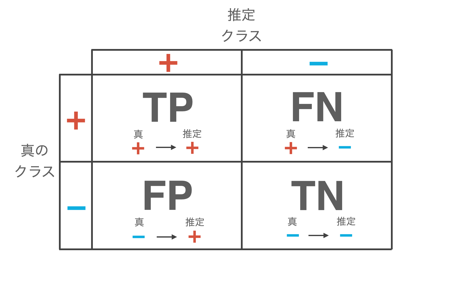
The most important aspect of addressing imbalanced data is understanding the cost of False Positives and False Negatives in the business context.
- Taking fraud detection as an example, false positives mean incorrectly flagging normal transactions as fraud, which creates customer inconvenience and customer support costs. On the other hand, false negatives mean missing fraud, which leads to direct monetary losses.
- In medical diagnosis examples, false positives misdiagnose healthy people as having a disease, resulting in unnecessary detailed examinations and psychological burden, while false negatives miss diseases, leading to lost treatment opportunities and risk of worsening conditions.
These costs are asymmetric, and in many cases, one is more severe than the other. Therefore, the optimization objective of machine learning models must reflect this asymmetric cost structure.
Evaluation Metric Selection: Critical Analysis and Practical Judgment
Why Accuracy is Inappropriate
Using only Accuracy for imbalanced data is problematic. In a dataset with 1% positive and 99% negative, a simple classifier that “always predicts negative” achieves 99% Accuracy. In other words, even a model that has learned nothing at all can achieve high Accuracy.
Expressed mathematically, $\text{Accuracy} = \frac{\text{TP} + \text{TN}}{\text{TP} + \text{TN} + \text{FP} + \text{FN}}$, but with imbalanced data, since the value of $\text{TN}$ (true negatives) is overwhelmingly large, changes in $\text{TP}$ or $\text{FP}$ have very little impact on Accuracy.
Precision, Recall, F1-Score: Practical Examples of Usage
Precision represents the proportion of actual positives among those predicted as positive, calculated as $\text{Precision} = \frac{\text{TP}}{\text{TP} + \text{FP}}$. This is a metric to emphasize when the cost of false positives is high, such as in spam filters or investment recommendation systems.
On the other hand, Recall (sensitivity) represents the proportion correctly detected among actual positives, calculated as $\text{Recall} = \frac{\text{TP}}{\text{TP} + \text{FN}}$. This is a metric to emphasize when the cost of false negatives is high, such as in cancer screening or fraud detection.
The F1-Score is the harmonic mean of Precision and Recall, calculated as $F_1 = \frac{2 \times \text{Precision} \times \text{Recall}}{\text{Precision} + \text{Recall}}$. However, the F1-Score has an important constraint: it places equal weight on Precision and Recall. In practical work, as mentioned earlier, the costs of false positives and false negatives are typically asymmetric.
To address this problem, the F-beta Score is used. \begin{align*} F_{\beta} = \frac{(1 + \beta^2) \times \text{Precision} \times \text{Recall}}{\beta^2 \times \text{Precision} + \text{Recall}} \end{align*} expressed by this equation, the weight can be adjusted by the value of $\beta$. When $\beta < 1$, Precision is emphasized; when $\beta = 1$, it’s the same as F1-Score; and when $\beta > 1$, Recall is emphasized. For example, in cancer screening, the $F_2$-Score (emphasizing Recall twice as much) is commonly used. On the other hand, for target selection in marketing campaigns, the $F_{0.5}$-Score (emphasizing Precision) might be appropriate.

ROC-AUC vs PR-AUC
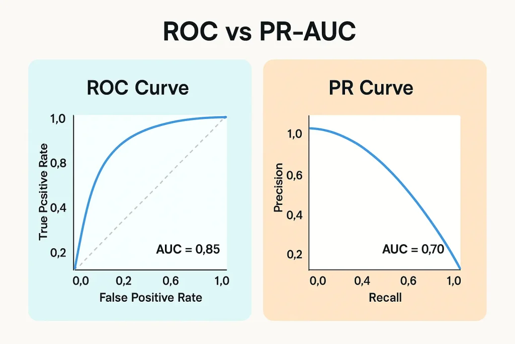
ROC-AUC (Area Under the ROC Curve) visualizes the trade-off between true positive rate ($\text{TPR} = \text{Recall}$) and false positive rate ($\text{FPR} = \frac{\text{FP}}{\text{FP}+\text{TN}}$) at different thresholds. However, using ROC-AUC for imbalanced data has a serious pitfall.
The denominator of FPR contains $\text{TN}$, but with imbalanced data, since the number of majority class samples is very large, even if you produce many false positives, FPR doesn’t increase much. For example, with 99% negative data, even if you incorrectly label 5% of negative samples as positive, FPR is only 0.05, which looks good on the ROC curve. However, in reality, a large number of false positives are occurring.
In contrast, PR-AUC (Area Under the Precision-Recall Curve) addresses this problem. Both Precision and Recall contain $\text{TP}$ in the numerator and don’t include the majority class $\text{TN}$ in the denominator, making it a more sensitive metric for imbalanced data. As a rule of thumb, when class balance is relatively good (e.g., 70:30 or better), AUC-ROC is also effective, but with extreme imbalance (90:10 or worse), PR-AUC should be prioritized. Additionally, it’s recommended to report both and pay particular attention to the PR-AUC value.
▼ Reference article

MCC (Matthews Correlation Coefficient)
MCC (Matthews Correlation Coefficient) is a type of correlation coefficient for binary classification that ranges from -1 to 1. \begin{align*} \text{MCC} = \frac{\text{TP} \times \text{TN} – \text{FP} \times \text{FN}}{\sqrt{(\text{TP}+\text{FP})(\text{TP}+\text{FN})(\text{TN}+\text{FP})(\text{TN}+\text{FN})}} \end{align*} calculated by this equation. The excellent feature of MCC is that it considers all four elements of the confusion matrix in a balanced way. It’s very robust for imbalanced data and provides comparable values even when class ratios change.
In practical work, MCC of 0.3 or higher can often be considered practical performance, and 0.5 or higher indicates good performance.
Linking to Business Metrics
Ultimately, technical metrics need to be translated into business metrics. The Expected Value Framework explicitly models the cost/benefit for each prediction outcome. \begin{align*} \text{Expected Value} = (\text{TP} \times \text{Benefit}_{\text{TP}}) + (\text{TN} \times \text{Benefit}_{\text{TN}}) – (\text{FP} \times \text{Cost}_{\text{FP}}) – (\text{FN} \times \text{Cost}_{\text{FN}}) \end{align*} expressed by this equation.
For example, in a fraud detection system, TP prevents an average loss of 100,000 yen by detecting fraud, TN correctly identifies normal transactions with near-zero cost, FP incorrectly flags normal transactions as fraud resulting in customer support costs of 3,000 yen, and FN misses fraud resulting in an average loss of 100,000 yen. Using this framework, you can directly compare the economic value of different models and threshold settings.
Data-Level Approaches: Systematic Understanding of Resampling Techniques
Data-level approaches directly manipulate the class distribution of training data. However, there is a large gap between practical work and academic research.
Undersampling Techniques
Undersampling is a technique that balances classes by reducing the number of majority class samples. In the simplest random undersampling, samples are randomly deleted from the majority class. This technique meets application conditions when the number of majority class samples is very large (hundreds of thousands or more). It’s also worth trying first as a baseline when computational resources are limited.
However, there’s a possibility of deleting important samples near the boundary, and since the number of samples is significantly reduced, the model’s generalization performance may deteriorate.
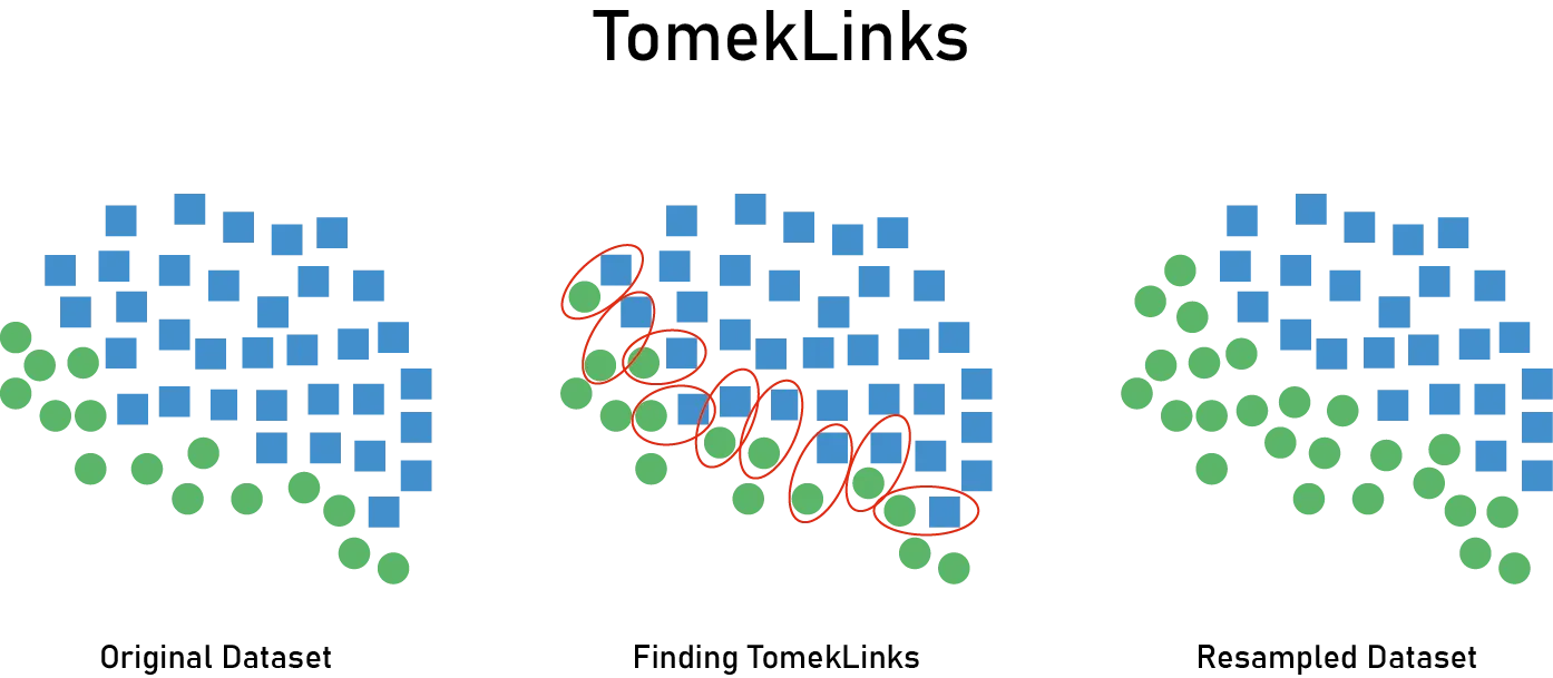
Tomek Links is a more sophisticated approach. A Tomek Link is a pair of samples that are mutual nearest neighbors and belong to different classes. By removing the majority class sample from this pair, noise near the decision boundary is removed. By removing ambiguous samples or label noise near class boundaries, clearer decision boundaries can be learned. However, the number of Tomek Links is often limited, making it insufficient for significant balance improvement. Also, nearest neighbor search becomes expensive in high-dimensional data.
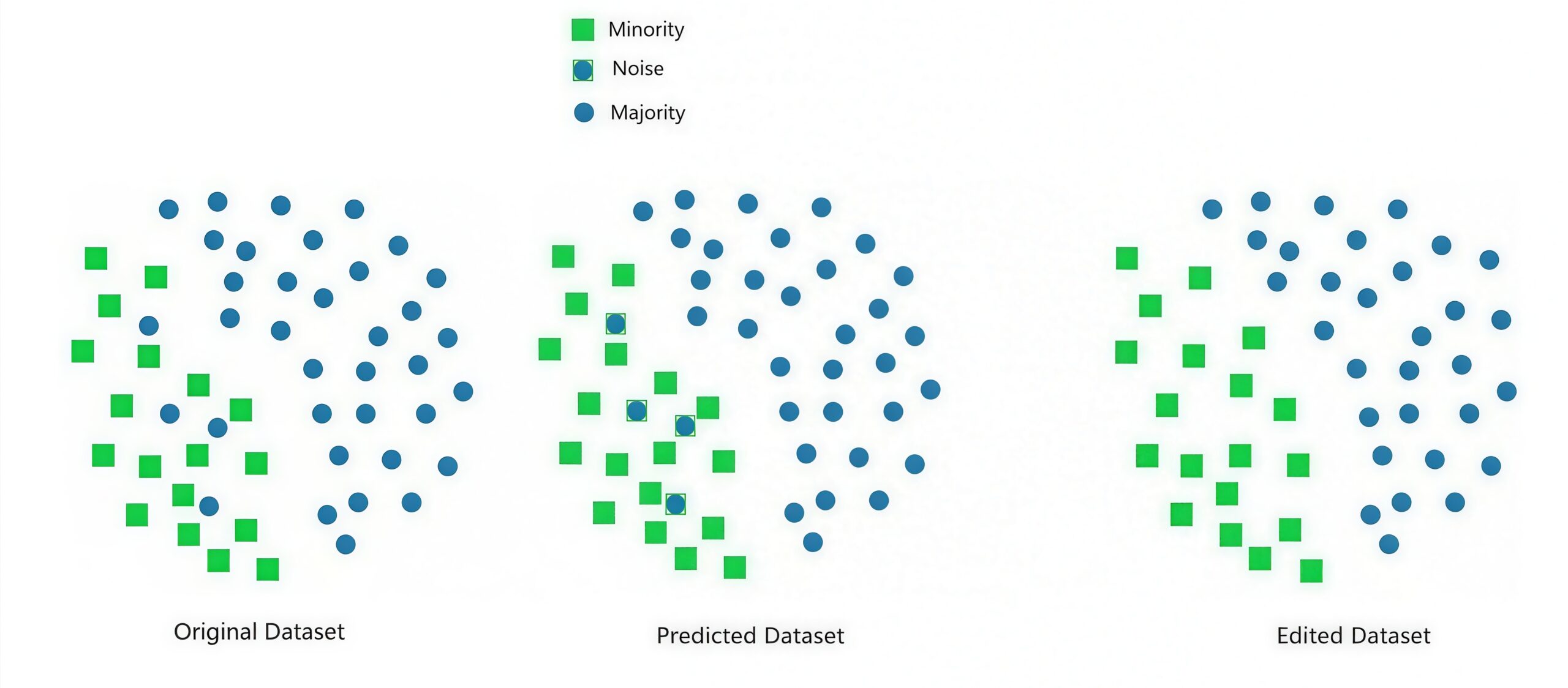
Edited Nearest Neighbors (ENN) examines the k-nearest neighbors of each sample and removes samples (mainly from the majority class) whose class doesn’t match by majority vote. It’s effective when there are many “intruder” samples from the majority class existing near the minority class, or when data contains noise. However, the choice of k significantly affects results, and since it removes samples more aggressively than Tomek Links, there’s a higher risk of information loss.
▼ Reference articles


Undersampling and Model Applicability Domain
An often-overlooked important aspect when applying undersampling is its impact on the Applicability Domain (AD) of the model. AD refers to the data region where the model can provide reliable predictions, and is defined by the distribution in the feature space of training data.
When you remove majority class samples, prediction accuracy (Precision/Recall) may improve while computational costs are also reduced. However, as a serious drawback that tends to be overlooked, the AD becomes narrower. For regions in feature space that were occupied by deleted samples, the model can no longer make reliable predictions. As a result, when samples outside the AD arrive in production environments, predictions become unreliable.
As a practical countermeasure, first, AD determination implementation is necessary. That is, implement a mechanism to determine whether new samples are within the AD. Next, decide how to handle samples outside the AD. Options include not returning predictions and referring to human judgment, attaching a low-confidence flag, or returning a default judgment (conservative decision). Furthermore, monitoring the proportion of samples outside the AD in production environments is important.
Methods for setting AD include k-nearest neighbor-based determination by distance to training data, learning the distribution of training data with One-Class SVM, using outlier scores with Isolation Forest, or measuring deviation from each feature’s distribution with standardized distance.
Let’s consider a fraud detection system as a specific case study. Normal transactions are diverse (various amounts, product categories, regions) while fraud is rare. With undersampling, if you reduce normal transactions in training data from 10,000 to 1,000 cases, the AD shrinks, and transaction patterns covered by the deleted 9,000 cases become outside the AD. As a result, production impact is that when transactions in that region arrive, the model cannot make reliable judgments. Consequently, 30% of all transactions may end up outside the AD, referred to human judgment, making the system not scalable.
On the other hand, with class_weight adjustment (discussed later), training data uses all 10,000 cases (with high weight for fraud), and the AD remains broad as originally. As a result, most transactions fall within the AD, enabling scalable automatic judgment.
SMOTE and the Gap with Practical Work
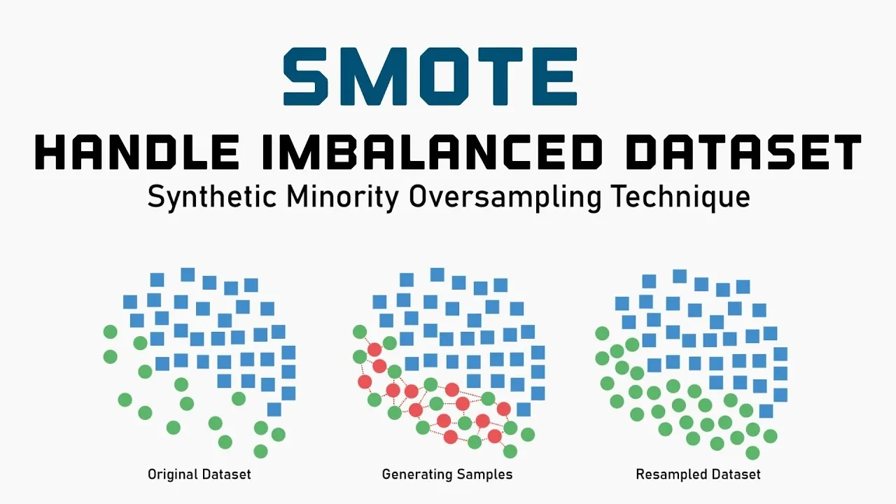
Ref: Balancing the Scales: How SMOTE Transforms Machine Learning with Imbalanced Data
SMOTE (Synthetic Minority Over-sampling Technique) generates synthetic samples by interpolating between minority class samples. Specifically, it randomly generates new samples on the line segment connecting a sample and its k-nearest neighbors. Theoretically, it’s intended to expand the minority class region in feature space and make decision boundaries smoother.
However, the reality in practical work is harsh, as SMOTE is rarely used in Kaggle top-winning solutions or actual production environments. This is also discussed in the data science community.
Why is it ineffective?
- There’s a fundamental problem of no information addition. SMOTE is merely interpolation of existing data and doesn’t add new information. It has almost equivalent effect to simple oversampling or weighting, while only increasing complexity.
- There’s a No Free Lunch theorem situation. Since it neither adds nor removes information, it can be effective or counterproductive depending on the case, and the average effect is close to zero.
- There’s a quality of synthesis problem. There’s no guarantee that nearest neighbor interpolation generates appropriate synthetic samples.
So what should be used? First, class_weight adjustment (discussed later) should be the top priority, as it’s simple and effective. Next, threshold optimization adjusts decision boundaries based on business costs. Also, when data is sufficiently large, undersampling can be considered, which also improves computational efficiency. And cost-sensitive learning directly addresses the essential problem (cost imbalance).
Oversampling and AD Issues
There’s an important recognition regarding oversampling: oversampling adds “fake samples.”
- First, there’s no information addition. It’s merely interpolation of existing data, and the AD doesn’t substantially expand.
- Second, there’s an illusion of incorrect AD expansion. The AD appears to have expanded with synthetic samples, but these are actually unvalidated regions.
- Third, there’s a reliability issue. Predictions in regions where synthetic samples are dense lack validation with real data.
As a practical recommendation, AD settings should be based on the original data before oversampling. Also, it’s important to distinguish regions of synthetic samples as “extended AD” and assign lower confidence to them.
Important Principles in Applying Resampling Techniques
- First, there’s an absolute rule: don’t resample validation data. If you resample validation or test data, you cannot evaluate the model’s true performance. Apply resampling only to training data.
- Second, the recognition that 50:50 is not necessarily optimal is important. The reason is it doesn’t reflect real-world distribution. In production environments, data arrives with a 1% vs 99% distribution, but learning with 50:50 distorts probability predictions. Also, excessive weighting of the minority class leads to overfitting and increased false positives. The recommended approach is to experiment in the range of 1:1 to 1:3, ultimately judging by cross-validation performance. Also consider applying probability calibration (Platt Scaling or Isotonic Regression) as post-processing.
- Third, the trade-off with data volume needs to be considered. Undersampling is only recommended when the number of majority class samples is sufficiently large. For example, with 1 million majority class samples and 10,000 minority class samples, undersampling still leaves 100,000 samples. However, with 10,000 majority class samples and 100 minority class samples, undersampling causes sample insufficiency.
Algorithm-Level Approaches
Algorithm-level approaches adapt the learning algorithm itself to imbalanced data rather than directly manipulating the data. In practical work, this is often more effective than data-level approaches.
Cost-Sensitive Learning (Class Weight Adjustment)
Cost-sensitive learning imposes larger penalties on misclassification of the minority class in the loss function, making the model pay attention to the minority class as well. Mathematically, as weighted cross-entropy loss,
\begin{align*}
\text{Loss} = -\frac{1}{N}\sum_{i=1}^{N} \left[ w_1 y_i \log(p_i) + w_0 (1-y_i)\log(1-p_i) \right]
\end{align*}
is expressed. Here, w1 (minority class weight) is set larger than w0 (majority class weight).
As a method for setting weights, there’s inverse frequency weighting, expressed by the following equation:
\begin{align*}
w_c = \frac{N}{K \cdot N_c}
\end{align*}
Here, $N$: total number of samples, $K$: number of classes ($K = 2$ for binary classification), $N_c$: number of samples of class $c$. For 1% vs 99%, the minority class weight becomes about 100 times. However, this can be too extreme.
In that case, there’s square root scaling,
\begin{align*}
w_c = \sqrt{\frac{N}{K \cdot N_c}}
\end{align*}
expressed by this equation. This is gentler weighting than inverse frequency weighting.
Alternatively, if actual business costs of misclassification are known,
\begin{align*}
w_0 = \frac{\text{Cost}_{\text{FN}}}{\text{Cost}_{\text{FP}} + \text{Cost}_{\text{FN}}}, \t w_1 = \frac{\text{Cost}_{\text{FP}}}{\text{Cost}_{\text{FP}} + \text{Cost}_{\text{FN}}}
\end{align*}
can be set this way.
$\text{Cost}_{\text{FN}}$ : Business cost when actually positive but predicted negative (False Negative)
$\text{Cost}_{\text{FP}}$ : Business cost when actually negative but predicted positive (False Positive)
As application conditions, it’s supported by most machine learning libraries (such as scikit-learn’s class_weight parameter), and implementation is simple since data resampling is unnecessary. Also, it’s particularly effective with stochastic gradient descent-based algorithms.
As constraints and cautions, there’s the danger of excessive weighting. If weights are made too large, each minority class sample exerts excessive influence, leading to overfitting. Furthermore, when using predicted probabilities directly in decision-making processes, output probabilities are distorted by weighting, requiring Probability Calibration.
Threshold Adjustment: Decision Boundary Optimization
Many classifiers use 0.5 as the default threshold. That is, if the predicted probability is 0.5 or higher, it’s judged positive; if lower, negative. However, for imbalanced data, this threshold is not optimal.
Theoretically, by adjusting the threshold, you can control the Precision-Recall trade-off.
- Lowering the threshold (e.g., 0.5 → 0.1) increases Recall and decreases Precision (predicting more as positive).
- Raising the threshold (e.g., 0.5 → 0.8) increases Precision and decreases Recall (predicting conservatively).
As methods for searching optimal thresholds, there’s F1-Score maximization. Calculate F1-Score at each threshold and select the threshold that maximizes it. This is appropriate when emphasizing balance.
There’s also business cost minimization, calculating expected cost at each threshold.
\begin{align*}
\text{Cost} = \text{FP} \times \text{Cost}_{\text{FP}} + \text{FN} \times \text{Cost}_{\text{FN}}
\end{align*}
by this equation, which is the recommended approach in practical work.
With Youden’s Index, maximize $J = \text{Sensitivity} + \text{Specificity} – 1$ and select the threshold closest to the top-left point on the ROC curve. Also, as securing specific Recall/Precision, conditions like “maximize Precision while securing Recall of 95% or higher” can be set.
As implementation notes, threshold search is performed on validation data and shouldn’t be used on test data. Whether to readjust thresholds in each fold of cross-validation or use one threshold overall depends on the situation. And when class distribution in production environments differs from training data, threshold readjustment is necessary.
Comparing cost-sensitive learning and threshold adjustment, both are worth trying. Cost-sensitive learning modifies the learning process itself, while threshold adjustment is post-processing. In practical work, combining both is also possible but needs to be done carefully.
One-Class Classification and Anomaly Detection Approach
For extreme imbalance (such as 99.9:0.1), reframing the problem as “anomaly detection” can be effective.
One-Class SVM learns only with the majority class (normal data) and detects samples that deviate from that distribution as anomalies (minority class). As application conditions, it’s effective when the number of minority class samples is extremely small (around tens), when minority class characteristics are diverse and supervised learning is difficult, and when normal data distribution is relatively compact. As constraints, hyperparameter tuning (especially the $\nu$ parameter) is difficult, and computational cost is high for large-scale data when using kernel tricks.
Isolation Forest randomly selects features and repeats splits, treating samples requiring fewer splits to isolate as anomalies. As a mechanism, anomaly samples are isolated in feature space so they can be isolated with fewer splits, while normal samples are dense so they require many splits. Advantages include being scalable and applicable to large-scale data, relatively robust to feature dimensionality, and having few hyperparameters. As application conditions, it’s effective when the minority class is truly “anomalous” (outlier-like) in feature space and when there’s large data volume. As a caution, effects are limited when the minority class is merely “rare” but not anomalous in feature space (e.g., similar distribution to majority class).
One-Class vs Two-Class: Which to Choose?
Cases where One-Class (anomaly detection) should be chosen include: imbalance ratio of 99.9:0.1 or higher, minority class labeled samples are tens or fewer, minority class characteristics are very diverse and cannot be represented by a few samples, and high possibility of new types of anomalies appearing in the future.
On the other hand, cases where Two-Class (regular classification) should be chosen include: imbalance ratio up to about 99:1, minority class samples are 100 or more, minority class characteristics are relatively consistent, and clear decision boundaries exist.
Model Architecture Selection
For imbalanced data, model architecture selection is as important as countermeasures. Since model behavior for imbalanced data varies greatly depending on the type, appropriate selection is key to success.
Tree-Based Model Characteristics
Tree-based models have multiple advantages. First, as decision boundary flexibility, they can express complex shapes by combining axis-parallel decision boundaries. Next, as sensitivity to minority class, they easily capture minority class clusters since they use leaf node purity as criterion. Furthermore, as scalability, XGBoost, LightGBM, and CatBoost are efficient for large-scale data.
As behavior with imbalanced data, purity criteria (Gini, Entropy) also respond to minority class samples. However, with extreme imbalance, the majority class is still dominant. Nevertheless, adjustment with scale_pos_weight (XGBoost) or class_weight (LightGBM) is effective.
As recommended settings, for XGBoost, start with scale_pos_weight around $\sqrt{\frac{\text{majority class count}}{\text{minority class count}}}$, start max_depth shallow (3-6) to prevent overfitting, and set min_child_weight larger to prevent minority class noise. For LightGBM, use is_unbalance=True or class_weight=’balanced’, and set min_data_in_leaf to about 1-5% of minority class sample count.
Neural Network Characteristics
Neural networks also have advantages. As expressive power, they can learn complex nonlinear relationships, and as high-dimensional data, they’re powerful for images, text, time series, etc. Also, as custom loss functions, losses specialized for imbalance like Focal Loss can be used.
As behavior with imbalanced data, gradient bias appears prominently, overfitting to majority class occurs easily, and standard techniques like batch normalization can become unstable under imbalance. Countermeasures are as follows:
- Focal Loss: This attenuates loss for easily classifiable samples. \begin{align*} \text{FL}(p_t) = -\alpha(1-p_t)^{\gamma} \log(p_t) \end{align*} expressed by this equation, start with $\gamma=2$ or so.
- Class-Balanced Loss: Weighting based on effective sample count, stable even with extreme imbalance.
- Two-stage training: Stage 1 pre-trains on resampled balanced data, Stage 2 fine-tunes on original imbalanced data.
Position of Linear Models
Linear models like Logistic Regression or Linear SVM have advantages of high interpretability, fast computation, and robustness to overfitting through regularization.
As challenges with imbalanced data, decision boundary expressiveness is limited, making them disadvantageous when minority class has complex distribution. As application conditions, they’re effective when feature engineering is sufficiently performed, classes are linearly separable or close to it, and interpretability is top priority.
As recommendations, use class_weight=’balanced’, carefully tune regularization parameter (C), and consider polynomial features or interaction terms.
Model Selection Flowchart
- As Step 1, check data characteristics. If sample count is under 10,000, consider tree-based or linear; 10,000 to 1 million, LightGBM/XGBoost; over 1 million, consider LightGBM or deep learning. As feature type, tabular data→tree-based, image/text→deep learning, mixed→start with tree-based.
- As Step 2, evaluate degree of imbalance. Up to 90:10, standard models and class_weight; up to 99:1, tree-based and class_weight, consider resampling; 99.9:0.1 or higher, also consider anomaly detection approach.
- As Step 3, consider business requirements. If interpretability is essential→linear models or shallow decision trees; if prediction accuracy is top priority→ensemble (XGBoost/LightGBM); if real-time prediction is needed→lightweight models (LightGBM or online learning).
Summary
Binary classification with imbalanced datasets is one of the challenges frequently encountered in practical machine learning work. This article explained approaches to address extreme imbalance such as 1% vs 99%.
As lessons learned, first, understanding the essence of the problem is important. The problem of imbalanced data is not simply the difference in class counts, but bias toward the majority class in loss function, gradients, and decision boundaries. This understanding becomes the foundation for selecting appropriate countermeasures.
Next, evaluation metrics. Accuracy alone is meaningless, and AUC-ROC is too optimistic. Evaluate with PR-AUC, Precision, Recall, and ultimately expected value based on business costs.
A stepwise approach is also important. First establish a baseline and add techniques one at a time to verify effects.
Emphasize practicality. Even with theoretically superior techniques, in practical work there are trade-offs with computational cost, implementation complexity, and maintainability. Start with simple and effective techniques like class_weight adjustment and threshold optimization. In fact, these techniques are proven in Kaggle top-winning solutions and products of major companies.
Finally, the most important thing in tackling imbalanced data problems is not application of technical methods, but deep understanding of business problems. What are the costs of false positives and false negatives, what kinds of judgment errors are most critical, what are the true needs of stakeholders—start by answering these questions.