


前言
K-Means 算法是最广为人知的聚类方法之一。K-Means 算法假设数据可以被分类为 $K$ 个簇,并按照一定的步骤将各个数据分配到其中一个簇中。
本文将介绍 K-Means 算法的机制及其实现方法。
此外,虽然 K-Means 算法需要预先给出要分类的簇数量,但本文也会介绍决定最佳簇数量的方法——肘部法则(Elbow Method)和轮廓分析(Silhouette Analysis)。
本文的源代码可以在以下的 Google Colab 中进行尝试。

\begin{align*}
\newcommand{\mat}[1]{\begin{pmatrix} #1 \end{pmatrix}}
\newcommand{\f}[2]{\frac{#1}{#2}}
\newcommand{\pd}[2]{\frac{\partial #1}{\partial #2}}
\newcommand{\d}[2]{\frac{{\rm d}#1}{{\rm d}#2}}
\newcommand{\T}{\mathsf{T}}
\newcommand{\dis}{\displaystyle}
\newcommand{\eq}[1]{{\rm Eq}(\ref{#1})}
\newcommand{\n}{\notag\\}
\newcommand{\t}{\ \ \ \ }
\newcommand{\tt}{\t\t\t\t}
\newcommand{\argmax}{\mathop{\rm arg\, max}\limits}
\newcommand{\argmin}{\mathop{\rm arg\, min}\limits}
\def\l<#1>{\left\langle #1 \right\rangle}
\def\us#1_#2{\underset{#2}{#1}}
\def\os#1^#2{\overset{#2}{#1}}
\newcommand{\case}[1]{\{ \begin{array}{ll} #1 \end{array} \right.}
\newcommand{\s}[1]{{\scriptstyle #1}}
\newcommand{\c}[2]{\textcolor{#1}{#2}}
\newcommand{\ub}[2]{\underbrace{#1}_{#2}}
\end{align*}
K-Means 算法的核心思想
假设簇的数量为 2,我们将基于下图来解释 K-Means 算法的核心思想。下图引用自 PRML(Pattern Recognition and Machine Learning 2006)。
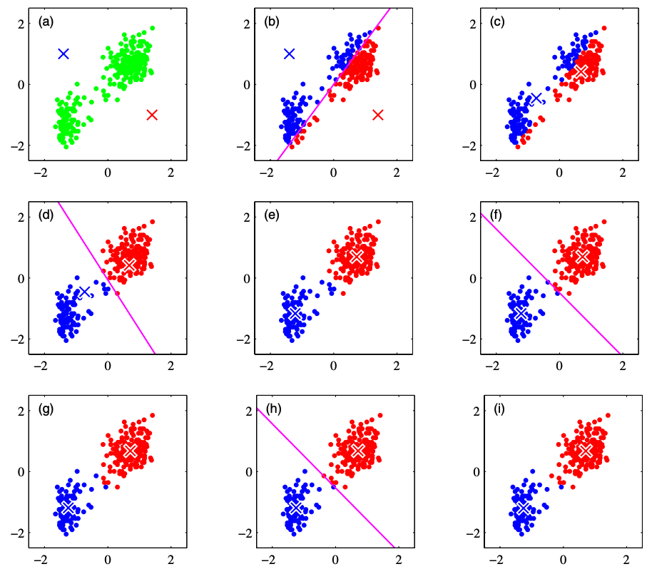
(a): 考虑每个簇的质心 $\bm{\mu}_1, \bm{\mu}_2$。现在,由于无法准确知道某个数据属于哪个簇,因此我们适当地给定簇质心的初始值。上图中红色和蓝色的叉号表示簇的质心。
(b): 根据每个数据距离哪个簇的质心更近,将其分配给相应的簇。
(c): 在分配好的簇内计算重心,并更新质心。
(d)~(i): 重复步骤 (b) 和 (c),持续更新簇。重复处理直到簇不再更新,或达到分析人员定义的最大迭代次数为止。
我们将上述过程公式化。
在 $N$ 个数据中,将第 $i$ 个数据点表示为 $\bm{x}^{(i)}$。此外,假设数据被分为 $K$ 个簇,将第 $j$ 个簇的质心表示为 $\bm{\mu}_j$。
那么,K-Means 算法就变成了以下损失函数的最小化问题。
\begin{align*}
L = \sum_{i=1}^N \sum_{j=1}^K r_{ij} \| \bm{x}^{(i)} – \bm{\mu}_j \|^2
\end{align*}
这里,$r_{ij}$ 是一个值,如果数据点 $x^{(i)}$ 属于第 $j$ 个簇,则取 $1$,否则取 $0$,
\begin{align*}
r_{ij} = \case{1\t {\rm if}\ j=\argmin_k \| \bm{x}^{(i)} – \bm{\mu}_k \|^2 \n 0 \t {\rm otherwise.}}
\end{align*}
可以这样表示。
另一方面,质心 $\bm{\mu}_j$ 的更新通过下式计算:
\begin{align*}
\bm{\mu}_j = \f{\sum_i r_{ij} \bm{x}^{(i)}}{\sum_i r_{ij}}
\end{align*}
从公式的形式可以看出,这实际上是在计算属于该簇的数据向量的平均值。
此外,上式也可以通过将损失函数关于 $\bm{\mu}_j$ 的偏导数设为 0,
\begin{align*}
\pd{L}{\bm{\bm{\mu}}_j} = 2 \sum_{i=1}^N r_{ij} (\bm{x}^{(i)} – \bm{\mu}_j) = 0
\end{align*}
并关于 $\bm{\mu}_j$ 求解得到。
因此,将 K-Means 算法的步骤公式化后,如下所示。
(a): 随机给出簇质心 $\bm{\mu}_j, (j=1, \dots, K)$ 的初始值。
(b):
\begin{align*}
r_{ij} = \case{1\t {\rm if}\ j=\argmin_k \| \bm{x}^{(i)} – \bm{\mu}_k \|^2 \n 0 \t {\rm otherwise.}}
\end{align*}
计算上式,将各数据分配给簇。
(c):
\begin{align*}
\bm{\mu}_j = \f{\sum_i r_{ij} \bm{x}^{(i)}}{\sum_i r_{ij}}
\end{align*}
计算上式,更新簇的质心。
(d): 重复步骤 (b) 和 (c),持续更新簇。重复处理直到簇不再更新,或达到分析人员定义的最大迭代次数为止。
K-Means 算法的实现
我们尝试使用 scikit-learn 进行基于 K-Means 算法的聚类分析。此外,本次使用的数据将使用 scikit-learn 的 make_blobs 生成用于分类的数据集。
首先创建分类用的数据集。
import numpy as np
import pandas as pd
import matplotlib.pyplot as plt
import seaborn as sns
from sklearn.datasets import make_blobs

X, y = make_blobs(
    n_samples=150,
    centers=3,
    cluster_std=1.0,
    shuffle=True,
    random_state=42)

x1 = X[:, 0]
x2 = X[:, 1]

plt.scatter(x1, x2)
plt.xlabel('x1')
plt.ylabel('x2')
plt.show()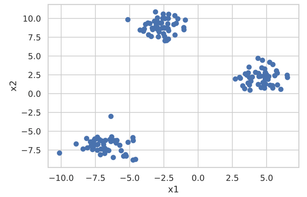
scikit-learn 提供了 sklearn.cluster.KMeans 类作为执行 K-Means 聚类分析的类。实现非常简单,如下所示。需要注意的是,必须预先确定要划分的簇数量。
from sklearn.cluster import KMeans

model = KMeans(n_clusters=3, random_state=0, init='random')  # If init is omitted, k-means++ is applied ('random' applies standard k-means)

model.fit(X)

clusters = model.predict(X)  # Get the cluster labels for the data

print(clusters)

# You can get the coordinates of the cluster centers with model.cluster_centers_
df_cluster_centers = pd.DataFrame(model.cluster_centers_)

df_cluster_centers.columns = ['x1', 'x2']

print(df_cluster_centers)## Outputs
[2 2 0 1 0 1 2 2 0 1 0 0 1 0 1 2 0 2 1 1 2 0 1 0 1 0 0 2 0 1 1 2 0 0 1 1 0
0 1 2 2 0 2 2 1 2 2 1 2 0 2 1 1 2 2 0 2 1 0 2 0 0 0 1 1 1 1 0 1 1 0 2 1 2
2 2 1 1 1 2 2 0 2 0 1 2 2 1 0 2 0 2 2 0 0 1 0 0 2 1 1 1 2 2 1 2 0 1 2 0 0
2 1 0 0 1 0 1 0 2 0 0 1 0 2 0 0 1 1 0 2 2 1 1 2 1 0 1 1 0 2 2 0 1 2 2 0 2
2 1]
x1 x2
0 -6.753996 -6.889449
1 4.584077 2.143144
2 -2.701466 8.902879光看这些很难理解,所以我们将聚类结果图示化。
df = pd.DataFrame(X, columns=['x1', 'x2'])
df['class'] = clusters

# Plot the clustered data
sns.scatterplot(data=df, x='x1', y='x2', hue='class')
# Plot the cluster centers
sns.scatterplot(data=df_cluster_centers, x='x1', y='x2', s=200, marker='*', color='gold', linewidth=0.5)
plt.show()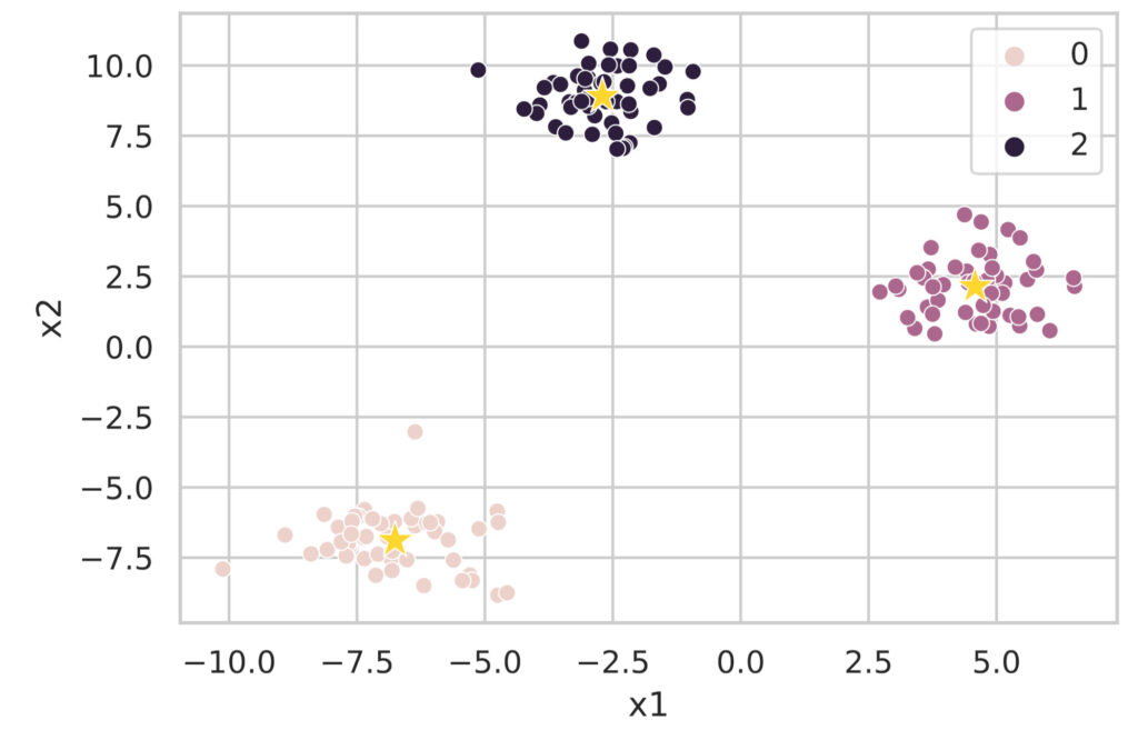
像这样,使用 sklearn.cluster.KMeans 类可以轻松执行基于 K-Means 算法的聚类分析。
探索最佳簇数量
K-Means 算法的一个问题是必须指定簇的数量。这里介绍用于确定最佳簇数量的肘部法则(Elbow Method)和轮廓分析(Silhouette Analysis)。另外,以下使用的数据是刚才用 make_blobs 创建的簇数量为 3 的数据。
肘部法则
肘部法则通过改变簇的数量,同时计算 K-Means 算法的损失函数
\begin{align*}
L = \sum_{i=1}^N \sum_{j=1}^K r_{ij} \| \bm{x}^{(i)} – \bm{\mu}_j \|^2
\end{align*}
并将结果图示化来确定最佳簇数量。
下面记载了肘部法则的实现。损失函数的值可以通过 model.inertia_ 访问。
# Execute the Elbow Method
sum_of_squared_errors = []

for i in range(1, 11):
    model = KMeans(n_clusters=i, random_state=0, init='random')
    model.fit(X)
    sum_of_squared_errors.append(model.inertia_)  # Store the value of the loss function

plt.plot(range(1, 11), sum_of_squared_errors, marker='o')
plt.xlabel('number of clusters')
plt.ylabel('sum of squared errors')
plt.show()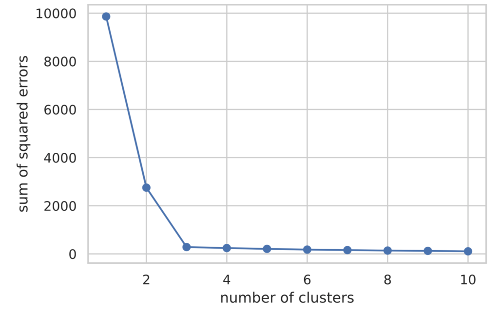
从图示结果可以看出,直到簇数量(横轴的值)为 3 时,损失函数的值都在减少,此后基本持平。
在肘部法则中,将损失函数减少程度急剧变化的簇数量判断为最佳簇数量。因此,可以判断本次情况下的最佳簇数量为 3。
轮廓分析
在轮廓分析中,基于以下指标来评价聚类的性能。
- 簇内的数据点越密集越好
- 各簇之间的距离越远越好
具体来说,通过按以下步骤定义的轮廓系数 (silhouette coefficient) 来评价聚类的性能。
(1) 作为簇内的凝聚度 $a^{(i)}$,计算某个数据点 $\bm{x}^{(i)}$ 与其所属簇 $C_{\rm in}$ 内的其他数据点的平均距离。
\begin{align*}
a^{(i)} = \f{1}{|C_{\rm in}| – 1} \sum_{\bm{x}^{(j)} \in C_{\rm in}} \| \bm{x}^{(i)} – \bm{x}^{(j)} \|
\end{align*}
(2) 作为与另一个簇的分离度 $b^{(i)}$,计算数据点 $\bm{x}^{(i)}$ 到距离最近的簇 $C_{\rm near}$ 所属数据点的平均距离。
\begin{align*}
b^{(i)} = \f{1}{|C_{\rm near}|} \sum_{\bm{x}^{(j)} \in C_{\rm near}} \| \bm{x}^{(i)} – \bm{x}^{(j)} \|
\end{align*}
(3) 用 $a^{(i)}$, $b^{(i)}$ 中较大的一个去除 $b^{(i)} – a^{(i)}$,计算轮廓系数 $s^{(i)}$。
\begin{align*}
s^{(i)} = \f{b^{(i)} – a^{(i)}}{\max(a^{(i)}, b^{(i)})}
\end{align*}
根据定义,轮廓系数落在 $[−1,1]$ 的区间内。此外,计算所有数据的轮廓系数并取平均值时,越接近 1 说明聚类性能越好。
轮廓分析的可视化遵循以下规则。
- 按所属簇编号排序
- 在同一簇内,按轮廓系数的值排序
通过将横轴设为轮廓系数,纵轴设为簇编号进行绘图,来实现轮廓分析的可视化。
import matplotlib.cm as cm
from sklearn.metrics import silhouette_samples

def show_silhouette(fitted_model):
    cluster_labels = np.unique(fitted_model.labels_)
    num_clusters = cluster_labels.shape[0]
    silhouette_vals = silhouette_samples(X, fitted_model.labels_)  # Calculate silhouette coefficients

    # Visualization
    y_ax_lower, y_ax_upper = 0, 0
    y_ticks = []

    for idx, cls in enumerate(cluster_labels):
        cls_silhouette_vals = silhouette_vals[fitted_model.labels_==cls]
        cls_silhouette_vals.sort()
        y_ax_upper += len(cls_silhouette_vals)
        cmap = cm.get_cmap("Spectral")
        rgba = list(cmap(idx/num_clusters))  # RGBA array
        rgba[-1] = 0.7  # Set alpha value to 0.7
        plt.barh(
            y=range(y_ax_lower, y_ax_upper),
            width=cls_silhouette_vals,
            height=1.0,
            edgecolor='none',
            color=rgba)
        y_ticks.append((y_ax_lower + y_ax_upper) / 2.0)
        y_ax_lower += len(cls_silhouette_vals)

    silhouette_avg = np.mean(silhouette_vals)
    plt.axvline(silhouette_avg, color='orangered', linestyle='--')
    plt.xlabel('silhouette coefficient')
    plt.ylabel('cluster')
    plt.yticks(y_ticks, cluster_labels + 1)
    plt.show()


for i in range(2, 5):
    model = KMeans(n_clusters=i, random_state=0, init='random')
    model.fit(X)
    show_silhouette(model)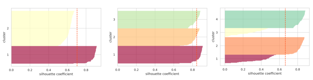
我们分别绘制了指定簇数量为 2, 3, 4 时的轮廓图。红色虚线表示轮廓系数的平均值。
如果簇分离得当,各簇轮廓的“厚度”往往会比较均匀。
就上图而言,可以看出簇数量为 3 时轮廓的“厚度”是均匀的,且轮廓系数的平均值最高。由此可以判断最佳簇数量为 3。
如上所述,在 scikit-learn 中可以简单地实现 K-Means 算法。
虽然必须预先给出要分类的簇数量,但我们介绍了作为决定簇数量的指导方针的肘部法则和轮廓分析。
此外,还有无需预先给出分类簇数量即可进行聚类的 X-Means 算法和 G-Means 算法。