


前言
本文将介绍机器学习中历史悠久的线性回归,特别是关于“最小二乘法”的理论及其 Python 实现。最小二乘法虽然模型简单,但具有广泛的应用和扩展性,是一种非常重要的思想。
例如,当我们观察散点图时,经常会觉得其中似乎存在某种直线关系。使用最小二乘法,就可以拟合出一条合适的直线。
(当然,有时也会觉得存在曲线关系,但本文将仅限于讨论直线关系。)
此外,本文的示例代码可以在以下链接中尝试。

\begin{align*}
\newcommand{\mat}[1]{\begin{pmatrix} #1 \end{pmatrix}}
\newcommand{\f}[2]{\frac{#1}{#2}}
\newcommand{\pd}[2]{\frac{\partial #1}{\partial #2}}
\newcommand{\d}[2]{\frac{{\rm d}#1}{{\rm d}#2}}
\newcommand{\T}{\mathsf{T}}
\newcommand{\dis}{\displaystyle}
\newcommand{\eq}[1]{{\rm Eq}(\ref{#1})}
\newcommand{\n}{\notag\\}
\newcommand{\t}{\ \ \ \ }
\newcommand{\tt}{\t\t\t\t}
\newcommand{\argmax}{\mathop{\rm arg\, max}\limits}
\newcommand{\argmin}{\mathop{\rm arg\, min}\limits}
\def\l<#1>{\left\langle #1 \right\rangle}
\def\us#1_#2{\underset{#2}{#1}}
\def\os#1^#2{\overset{#2}{#1}}
\newcommand{\case}[1]{\{ \begin{array}{ll} #1 \end{array} \right.}
\newcommand{\s}[1]{{\scriptstyle #1}}
\newcommand{\c}[2]{\textcolor{#1}{#2}}
\newcommand{\ub}[2]{\underbrace{#1}_{#2}}
\end{align*}
捕捉两个变量之间的关系
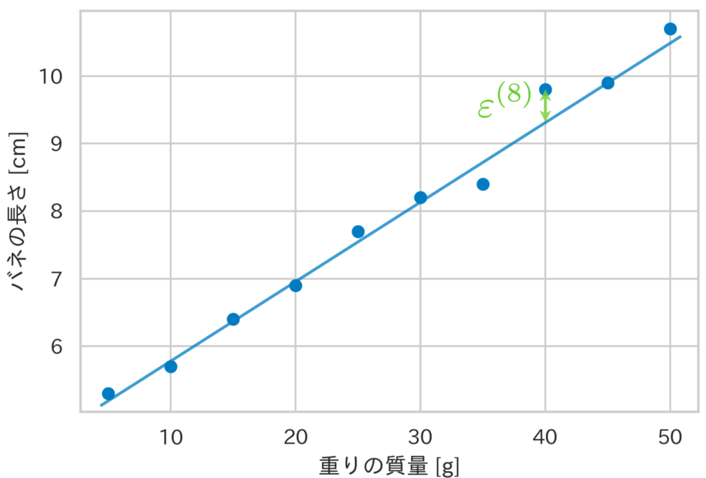
这里以悬挂在弹簧上的“重物质量”与“弹簧长度”之间的关系为例。下面展示了10组重物质量和弹簧长度的数据及其散点图。
| 重物质量 [g] | 弹簧长度 [cm] |
|---|---|
| 5 | 5.3 |
| 10 | 5.7 |
| 15 | 6.4 |
| 20 | 6.9 |
| 25 | 7.7 |
| 30 | 8.2 |
| 35 | 8.4 |
| 40 | 9.8 |
| 45 | 9.9 |
| 50 | 10.7 |

假设重物质量 $x$ 和弹簧长度 $y$ 这两个变量之间存在
\begin{align*}
y = u(x)
\end{align*}
这样的关系。
现在,让我们考虑表示该现象真实结构的未知函数 $u(x)$。根据数据趋势或先验知识,我们假设*该现象的结构是线性的,即它是一条直线。
因此,作为真实结构 $u(x)$,
\begin{align*}
y = u(x) = \theta_0 + \theta_1 x
\end{align*}
我们设想如上式。如果该现象的结构确实是线性的,且表1中的数据不存在误差,那么只要恰当地确定直线的截距 $\theta_0$ 和斜率 $\theta_1$,这10个数据点将全部落在一条直线上。
然而,实际上由于误差的影响,数据会偏离该直线。因此,我们考虑到这个偏差 $\varepsilon$,假设满足关系式 $y = \theta_0 + \theta_1 x + \varepsilon$。
一般而言,当观测到 $n$ 个数据时,第 $i$ 个数据点 $(x^{(i)}, y^{(i)})$ 满足下式(规定将索引 $i$ 标记在右上角)。
\begin{align*}
y^{(i)} = \theta_0 + \theta_1 x^{(i)} + \varepsilon^{(i)}.
\end{align*}
这里,$\theta_0, \theta_1$ 称为回归系数,$\varepsilon^{(i)}$ 称为误差项,由上式表示的模型称为线性回归模型。此外,相当于弹簧长度的变量 $y$ 被称为目标变量,相当于重物质量的变量 $x$ 被称为解释变量。
那么,应该如何确定回归系数 $\theta_0, \theta_1$ 呢?确定这些参数值的方法之一就是最小二乘法。
*假设存在曲线关系,模型可能会变成例如 $y=\theta_0 + \theta_1 x + \theta_2 x^2 + \varepsilon$ 的形式。不过,即使在这种情况下,由于目标变量关于参数 $\theta$ 是线性的,因此仍归类为线性回归问题。也就是说,如果设 $\bm{x} = (1, x, x^2)^\T$, $\bm{\theta} = (\theta_0, \theta_1, \theta_2)^\T$,则 $y = \bm{\theta}^\T \bm{x} + \varepsilon$ 是线性的。因此,求解 $\bm{\theta}$ 的估计值与下一节的方法没有太大区别。
使用最小二乘法估计回归系数
在本次的线性回归模型中,我们认为第 $i$ 个数据 $x^{(i)}$ 的真实值是 $\theta_0 + \theta_1 x^{(i)}$,在此基础上加上误差 $\varepsilon^{(i)}$ 后,观测到了数据 $y^{(i)}$。
最小二乘法是一种通过使各数据的误差项的平方和 $(\varepsilon^{(1)})^2 + (\varepsilon^{(2)})^2 + \cdots + (\varepsilon^{(n)})^2$ 最小化来确定回归系数 $\theta_0, \theta_1$ 的方法。现在,因为 $\varepsilon^{(i)} = y^{(i)} – (\theta_0 + \theta_1 x^{(i)})$,如果用数学公式表达最小二乘法,定义平方和为 $J \equiv \sum_i (\varepsilon^{(i)})^2$,则可以表示为下式。
\begin{align*}
\{\theta_0, \theta_1\} &= \argmin_{\theta_0, \theta_1} J(\theta_0, \theta_1) \n
&= \argmin_{\theta_0, \theta_1} \sum_{i=1}^n (\varepsilon^{(i)})^2 \n
&= \argmin_{\theta_0, \theta_1} \sum_{i=1}^n \[ y^{(i)} – (\theta_0 + \theta_1 x^{(i)}) \]^2.
\end{align*}
因此,我们将 $J(\theta_0, \theta_1)$ 视为回归系数 $\theta_0, \theta_1$ 的函数,通过令偏导数为0,求出使 $J$ 最小的回归系数的值。
\begin{align*}
J(\theta_0, \theta_1) = \sum_{i=1}^n \[ y^{(i)} – (\theta_0 + \theta_1 x^{(i)}) \]^2
\end{align*}
由上式得,
\begin{align*}
\pd{J}{\theta_0} = 2 \sum_{i=1}^n \(y^{(i)} – \theta_0 – \theta_1 x^{(i)} \) \cdot (-1) = 0 \n
\therefore \sum_{i=1}^n y^{(i)} = \sum_{i=1}^n \theta_0 + \sum_{i=1}^n \theta_1 x^{(i)},
\end{align*}
\begin{align*}
\pd{J}{\theta_1} = 2 \sum_{i=1}^n \[ \(y^{(i)} – \theta_0 – \theta_1 x^{(i)} \) \cdot (-x^{(i)}) \] = 0 \n
\therefore \sum_{i=1}^n x^{(i)}y^{(i)} = \sum_{i=1}^n \theta_0 x^{(i)} + \sum_{i=1}^n \theta_1 (x^{(i)})^2.
\end{align*}
综上所述,解下列联立方程组即可求得回归系数的估计值 $\hat{\theta}_0, \hat{\theta}_1$。
\begin{align*}
\case{
\sum_i y^{(i)} = n \theta_0 + \theta_1 \sum_i x^{(i)}, \\
\sum_i x^{(i)}y^{(i)} = \theta_0 \sum_i x^{(i)} + \theta_1 \sum_i (x^{(i)})^2. }
\end{align*}
利用期望值 ${\rm E}[x] = \f{1}{n} \sum_i x^{(i)}$ 进行整理,得
\begin{align*}
\case{
{\rm E}[y] = \theta_0 + \theta_1 {\rm E}[x], \\
{\rm E}[xy] = \theta_0 {\rm E}[x] + \theta_1 {\rm E}[x^2]. }
\end{align*}
因此,作为联立方程组解的回归系数估计值 $\hat{\theta}_0, \hat{\theta}_1$ 分别为,
\begin{align*}
\hat{\theta}_0 = {\rm E}[y] – \hat{\theta_1} {\rm E}[x], \t \hat{\theta}_1 &= \f{{\rm E}[xy] – {\rm E}[x] \cdot {\rm E}[y]}{{\rm E}[x^2] – {\rm E}[x]^2} \n
&= \f{{\rm Cov}(x, y)}{{\rm V}[x]} \t (☆)
\end{align*}
计算得出。这里,${\rm{V}}[x]$ 表示方差,${\rm Cov}(x, y)$ 表示协方差。
使用 Python 计算回归系数
我们要尝试使用 Python 计算回归系数。示例使用文章开头展示的悬挂在弹簧上的重物质量与弹簧长度的关系。其实要做的事情很简单,只需计算式(☆)即可。
import numpy as np
import matplotlib.pyplot as plt

weights = np.array([5, 10, 15, 20, 25, 30, 35, 40, 45, 50])
lengths = np.array([5.3, 5.7, 6.4, 6.9, 7.7, 8.2, 8.4, 9.8, 9.9, 10.7])


def least_squares(x, y):
    """回帰係数を計算する"""
    theta_1 = np.cov(x, y)[0][1] / np.var(x)
    theta_0 = np.mean(y) - theta_1 * np.mean(x)
    return theta_0, theta_1


theta_0, theta_1 = least_squares(weights, lengths)

print(f'切片: {theta_0}')
print(f'傾き: {theta_1}')


x = np.arange(5, 55, 0.1)
y = theta_0 + theta_1 * x  # 回帰曲線
# 可視化
plt.scatter(weights, lengths, c='#007bc3')
plt.plot(x, y, c='#de3838')
plt.show()## 出力
切片: 4.196296296296298
傾き: 0.13468013468013465
使用 scikit-learn 计算回归系数
同样也可以使用 scikit-learn 求解回归系数。
from sklearn.linear_model import LinearRegression

weights = np.array([5, 10, 15, 20, 25, 30, 35, 40, 45, 50])
lengths = np.array([5.3, 5.7, 6.4, 6.9, 7.7, 8.2, 8.4, 9.8, 9.9, 10.7])

model = LinearRegression()
model.fit(weights.reshape(-1, 1), lengths)

theta_0, theta_1 = model.intercept_, model.coef_

print(f'切片: {theta_0}')
print(f'傾き: {theta_1}')


x = np.arange(5, 55, 0.1)
y = theta_0 + theta_1 * x  # 回帰曲線

# 可視化
plt.scatter(weights, lengths, c='#007bc3')
plt.plot(x, y, c='#de3838')
plt.show()## 出力
切片: 4.566666666666668
傾き: [0.12121212]
多元回归分析的讲解请见此处▼