


Introduction
One of the most well-known clustering methods is the k-means method. The k-means method assumes that data can be classified into $K$ clusters, and assigns each data point to one of the clusters according to a specific procedure.
In this article, I will discuss the mechanism of the k-means method and how to implement it.
Additionally, while the k-means method requires the number of clusters to be specified in advance, I will introduce the Elbow Method and Silhouette Analysis as methods for determining the optimal number of clusters.
The source code for this article can be tried out on Google Colab below.

\begin{align*}
\newcommand{\mat}[1]{\begin{pmatrix} #1 \end{pmatrix}}
\newcommand{\f}[2]{\frac{#1}{#2}}
\newcommand{\pd}[2]{\frac{\partial #1}{\partial #2}}
\newcommand{\d}[2]{\frac{{\rm d}#1}{{\rm d}#2}}
\newcommand{\T}{\mathsf{T}}
\newcommand{\dis}{\displaystyle}
\newcommand{\eq}[1]{{\rm Eq}(\ref{#1})}
\newcommand{\n}{\notag\\}
\newcommand{\t}{\ \ \ \ }
\newcommand{\tt}{\t\t\t\t}
\newcommand{\argmax}{\mathop{\rm arg\, max}\limits}
\newcommand{\argmin}{\mathop{\rm arg\, min}\limits}
\def\l<#1>{\left\langle #1 \right\rangle}
\def\us#1_#2{\underset{#2}{#1}}
\def\os#1^#2{\overset{#2}{#1}}
\newcommand{\case}[1]{\{ \begin{array}{ll} #1 \end{array} \right.}
\newcommand{\s}[1]{{\scriptstyle #1}}
\newcommand{\c}[2]{\textcolor{#1}{#2}}
\newcommand{\ub}[2]{\underbrace{#1}_{#2}}
\end{align*}
The Concept of k-means Clustering
Assuming the number of clusters is 2, I will explain the concept of the k-means method based on the figure below. The figure is cited from PRML (Pattern Recognition and Machine Learning 2006).
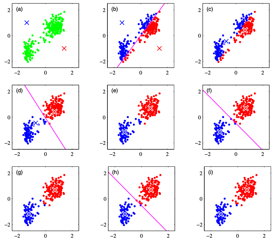
(a): Consider centroids $\bm{\mu}_1, \bm{\mu}_2$ for each cluster. Since we do not currently know exactly which cluster a given data point belongs to, we assign the initial values of the cluster centroids arbitrarily. In the figure above, the red and blue crosses indicate the cluster centroids.
(b): Assign each data point to a cluster based on which cluster centroid it is closer to.
(c): Within the assigned clusters, calculate the centroid and update the centroid position.
(d)~(i): Repeat steps (b) and (c) to continue updating the clusters. The iterative process continues until there are no more cluster updates or until the maximum number of iterations defined by the analyst is reached.
Let’s formulate the above.
Out of $N$ data points, let the $i$-th data point be denoted as $\bm{x}^{(i)}$. Also, assuming this data is divided into $K$ clusters, let the centroid of the $j$-th cluster be denoted as $\bm{\mu}_j$.
Then, the k-means method becomes a minimization problem of the following loss function:
\begin{align*}
L = \sum_{i=1}^N \sum_{j=1}^K r_{ij} \| \bm{x}^{(i)} – \bm{\mu}_j \|^2
\end{align*}
Here, $r_{ij}$ takes the value $1$ if the data point $x^{(i)}$ belongs to the $j$-th cluster, and $0$ otherwise, which can be expressed as:
\begin{align*}
r_{ij} = \case{1\t {\rm if}\ j=\argmin_k \| \bm{x}^{(i)} – \bm{\mu}_k \|^2 \n 0 \t {\rm otherwise.}}
\end{align*}
On the other hand, the update of the centroid $\bm{\mu}_j$ is calculated by:
\begin{align*}
\bm{\mu}_j = \f{\sum_i r_{ij} \bm{x}^{(i)}}{\sum_i r_{ij}}
\end{align*}
From the form of the equation, it can be seen that this calculates the mean value of the data vectors belonging to the cluster.
Also, the above equation is obtained by setting the partial derivative of the loss function with respect to $\bm{\mu}_j$ to 0,
\begin{align*}
\pd{L}{\bm{\bm{\mu}}_j} = 2 \sum_{i=1}^N r_{ij} (\bm{x}^{(i)} – \bm{\mu}_j) = 0
\end{align*}
and solving for $\bm{\mu}_j$.
Therefore, the procedure of the k-means method can be formulated as follows:
(a): Randomly assign initial values for the cluster centroids $\bm{\mu}_j, (j=1, \dots, K)$.
(b): Calculate
\begin{align*}
r_{ij} = \case{1\t {\rm if}\ j=\argmin_k \| \bm{x}^{(i)} – \bm{\mu}_k \|^2 \n 0 \t {\rm otherwise.}}
\end{align*}
and assign each data point to a cluster.
(c): Calculate
\begin{align*}
\bm{\mu}_j = \f{\sum_i r_{ij} \bm{x}^{(i)}}{\sum_i r_{ij}}
\end{align*}
and update the cluster centroids.
(d): Repeat steps (b) and (c) to continue updating the clusters. The iterative process continues until there are no more cluster updates or until the maximum number of iterations defined by the analyst is reached.
Implementation of k-means Clustering
Let’s perform cluster analysis using the k-means method with scikit-learn. For the data, we will generate a dataset for classification using make_blobs from scikit-learn.
First, create the dataset for classification.
import numpy as np
import pandas as pd
import matplotlib.pyplot as plt
import seaborn as sns
from sklearn.datasets import make_blobs

X, y = make_blobs(
    n_samples=150,
    centers=3,
    cluster_std=1.0,
    shuffle=True,
    random_state=42)

x1 = X[:, 0]
x2 = X[:, 1]

plt.scatter(x1, x2)
plt.xlabel('x1')
plt.ylabel('x2')
plt.show()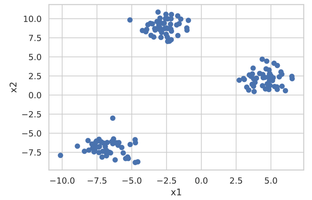
scikit-learn provides the sklearn.cluster.KMeans class for performing cluster analysis using the k-means method. Implementation is extremely simple, as shown below. **Note that the number of clusters to divide into must be decided in advance.**
from sklearn.cluster import KMeans

model = KMeans(n_clusters=3, random_state=0, init='random')  # If init is omitted, k-means++ is applied ('random' applies standard k-means)

model.fit(X)

clusters = model.predict(X)  # Get the cluster labels for the data

print(clusters)

# You can get the coordinates of the cluster centers with model.cluster_centers_
df_cluster_centers = pd.DataFrame(model.cluster_centers_)

df_cluster_centers.columns = ['x1', 'x2']

print(df_cluster_centers)## Outputs
[2 2 0 1 0 1 2 2 0 1 0 0 1 0 1 2 0 2 1 1 2 0 1 0 1 0 0 2 0 1 1 2 0 0 1 1 0
0 1 2 2 0 2 2 1 2 2 1 2 0 2 1 1 2 2 0 2 1 0 2 0 0 0 1 1 1 1 0 1 1 0 2 1 2
2 2 1 1 1 2 2 0 2 0 1 2 2 1 0 2 0 2 2 0 0 1 0 0 2 1 1 1 2 2 1 2 0 1 2 0 0
2 1 0 0 1 0 1 0 2 0 0 1 0 2 0 0 1 1 0 2 2 1 1 2 1 0 1 1 0 2 2 0 1 2 2 0 2
2 1]
x1 x2
0 -6.753996 -6.889449
1 4.584077 2.143144
2 -2.701466 8.902879Since this alone is hard to understand, let’s visualize the clustering results.
df = pd.DataFrame(X, columns=['x1', 'x2'])
df['class'] = clusters

# Plot the clustered data
sns.scatterplot(data=df, x='x1', y='x2', hue='class')
# Plot the cluster centers
sns.scatterplot(data=df_cluster_centers, x='x1', y='x2', s=200, marker='*', color='gold', linewidth=0.5)
plt.show()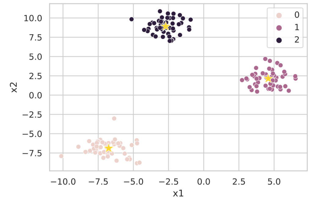
As you can see, cluster analysis using the k-means method can be easily executed with the sklearn.cluster.KMeans class.
Searching for the Optimal Number of Clusters
One of the problems with the k-means method is that you have to specify the number of clusters. Here, I will introduce the Elbow Method and Silhouette Analysis, which are used to determine the optimal number of clusters. The data used below is the data with 3 clusters created earlier with make_blobs.
Elbow Method
In the Elbow Method, we calculate the loss function of the k-means method while changing the number of clusters:
\begin{align*}
L = \sum_{i=1}^N \sum_{j=1}^K r_{ij} \| \bm{x}^{(i)} – \bm{\mu}_j \|^2
\end{align*}
and determine the optimal number of clusters by visualizing the results.
The implementation of the Elbow Method is described below. The value of the loss function can be accessed with model.inertia_.
# Execute the Elbow Method
sum_of_squared_errors = []

for i in range(1, 11):
    model = KMeans(n_clusters=i, random_state=0, init='random')
    model.fit(X)
    sum_of_squared_errors.append(model.inertia_)  # Store the value of the loss function

plt.plot(range(1, 11), sum_of_squared_errors, marker='o')
plt.xlabel('number of clusters')
plt.ylabel('sum of squared errors')
plt.show()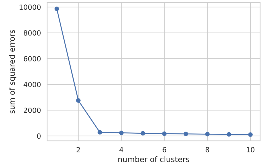
Looking at the plotted results, we can see that the value of the loss function decreases until the number of clusters (value on the horizontal axis) is 3, and after that, it remains almost flat.
In the Elbow Method, the number of clusters where the rate of decrease of the loss function changes rapidly is judged as the optimal number of clusters. Therefore, in this case, we can determine that the optimal number of clusters is 3.
Silhouette Analysis
In Silhouette Analysis, clustering performance is evaluated based on the following indicators:
- The denser the data points within a cluster, the better.
- The further apart each cluster is, the better.
Specifically, we evaluate clustering performance using the **silhouette coefficient** defined by the following procedure.
(1) As the **cohesion** $a^{(i)}$ within a cluster, calculate the average distance to other data points in the cluster $C_{\rm in}$ to which a certain data point $\bm{x}^{(i)}$ belongs.
\begin{align*}
a^{(i)} = \f{1}{|C_{\rm in}| – 1} \sum_{\bm{x}^{(j)} \in C_{\rm in}} \| \bm{x}^{(i)} – \bm{x}^{(j)} \|
\end{align*}
(2) As the **separation** $b^{(i)}$ from other clusters, calculate the average distance to data points belonging to the nearest cluster $C_{\rm near}$ to the data point $\bm{x}^{(i)}$.
\begin{align*}
b^{(i)} = \f{1}{|C_{\rm near}|} \sum_{\bm{x}^{(j)} \in C_{\rm near}} \| \bm{x}^{(i)} – \bm{x}^{(j)} \|
\end{align*}
(3) Calculate the **silhouette coefficient** $s^{(i)}$ by dividing $b^{(i)} – a^{(i)}$ by the larger of $a^{(i)}$ and $b^{(i)}$.
\begin{align*}
s^{(i)} = \f{b^{(i)} – a^{(i)}}{\max(a^{(i)}, b^{(i)})}
\end{align*}
From its definition, the silhouette coefficient falls within the interval $[−1,1]$. Also, when calculating the silhouette coefficient for all data and taking the average value, closer to 1 indicates better clustering performance.
Visualization of silhouette analysis follows these rules:
- Sort by assigned cluster number.
- Sort by silhouette coefficient value within the same cluster.
Silhouette analysis is visualized by plotting the silhouette coefficient on the horizontal axis and the cluster number on the vertical axis.
import matplotlib.cm as cm
from sklearn.metrics import silhouette_samples

def show_silhouette(fitted_model):
    cluster_labels = np.unique(fitted_model.labels_)
    num_clusters = cluster_labels.shape[0]
    silhouette_vals = silhouette_samples(X, fitted_model.labels_)  # Calculate silhouette coefficients

    # Visualization
    y_ax_lower, y_ax_upper = 0, 0
    y_ticks = []

    for idx, cls in enumerate(cluster_labels):
        cls_silhouette_vals = silhouette_vals[fitted_model.labels_==cls]
        cls_silhouette_vals.sort()
        y_ax_upper += len(cls_silhouette_vals)
        cmap = cm.get_cmap("Spectral")
        rgba = list(cmap(idx/num_clusters))  # RGBA array
        rgba[-1] = 0.7  # Set alpha value to 0.7
        plt.barh(
            y=range(y_ax_lower, y_ax_upper),
            width=cls_silhouette_vals,
            height=1.0,
            edgecolor='none',
            color=rgba)
        y_ticks.append((y_ax_lower + y_ax_upper) / 2.0)
        y_ax_lower += len(cls_silhouette_vals)

    silhouette_avg = np.mean(silhouette_vals)
    plt.axvline(silhouette_avg, color='orangered', linestyle='--')
    plt.xlabel('silhouette coefficient')
    plt.ylabel('cluster')
    plt.yticks(y_ticks, cluster_labels + 1)
    plt.show()


for i in range(2, 5):
    model = KMeans(n_clusters=i, random_state=0, init='random')
    model.fit(X)
    show_silhouette(model)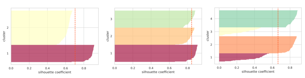
I plotted silhouette diagrams when the number of clusters was specified as 2, 3, and 4, respectively. The red dashed line represents the average value of the silhouette coefficients.
If the clusters are properly separated, the “thickness” of the silhouette for each cluster tends to be nearly uniform.
In the figure above, when the number of clusters is 3, the “thickness” of the silhouettes is uniform, and it can be seen that the average silhouette coefficient is the highest. From this, we can judge that the optimal number of clusters is 3.
Reference: scikit-learn official page
As described above, implementation of the k-means method can be easily performed in scikit-learn.
Although the number of clusters to be classified needs to be provided in advance, I introduced the Elbow Method and Silhouette Analysis as guidelines for determining that number.
Note that there are also methods called x-means and g-means that can perform clustering without providing the number of clusters in advance.