


Introduction
In this article, we will introduce the theory and Python implementation of the “Least Squares Method,” focusing on linear regression, which has a long history in machine learning. The Least Squares Method (also called the method of least squares) is a simple model but has many applications and developments, making it a very important concept.
For example, when looking at a scatter plot, we often think there might be a linear relationship. Using the Least Squares Method makes it possible to fit an appropriate line.
(Of course, we might sometimes think there is a curvilinear relationship, but here we will limit our discussion to linear relationships.)
Also, the sample code for this article can be tested below.

\begin{align*}
\newcommand{\mat}[1]{\begin{pmatrix} #1 \end{pmatrix}}
\newcommand{\f}[2]{\frac{#1}{#2}}
\newcommand{\pd}[2]{\frac{\partial #1}{\partial #2}}
\newcommand{\d}[2]{\frac{{\rm d}#1}{{\rm d}#2}}
\newcommand{\T}{\mathsf{T}}
\newcommand{\dis}{\displaystyle}
\newcommand{\eq}[1]{{\rm Eq}(\ref{#1})}
\newcommand{\n}{\notag\\}
\newcommand{\t}{\ \ \ \ }
\newcommand{\tt}{\t\t\t\t}
\newcommand{\argmax}{\mathop{\rm arg\, max}\limits}
\newcommand{\argmin}{\mathop{\rm arg\, min}\limits}
\def\l<#1>{\left\langle #1 \right\rangle}
\def\us#1_#2{\underset{#2}{#1}}
\def\os#1^#2{\overset{#2}{#1}}
\newcommand{\case}[1]{\{ \begin{array}{ll} #1 \end{array} \right.}
\newcommand{\s}[1]{{\scriptstyle #1}}
\newcommand{\c}[2]{\textcolor{#1}{#2}}
\newcommand{\ub}[2]{\underbrace{#1}_{#2}}
\end{align*}
Capturing the Relationship Between Two Variables
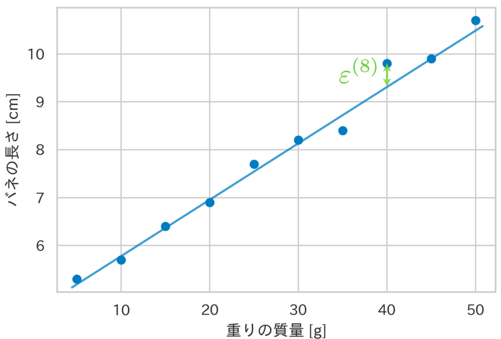
Here, we will take the relationship between the “mass of a weight” hung on a spring and the “length of the spring” as an example. Below, we show 10 sets of data for the weight’s mass and the spring’s length, along with their scatter plot.
| Mass of Weight [g] | Length of Spring [cm] |
|---|---|
| 5 | 5.3 |
| 10 | 5.7 |
| 15 | 6.4 |
| 20 | 6.9 |
| 25 | 7.7 |
| 30 | 8.2 |
| 35 | 8.4 |
| 40 | 9.8 |
| 45 | 9.9 |
| 50 | 10.7 |

Assume there is a relationship between the two variables, weight mass $x$ and spring length $y$, given by
\begin{align*}
y = u(x)
\end{align*}
as shown above.
Now, let’s consider the unknown function $u(x)$ representing the true structure of this phenomenon. Based on data trends or a priori knowledge, we **assume*** that the structure of this phenomenon is linear, that is, it might be a straight line.
Thus, for the true structure $u(x)$,
\begin{align*}
y = u(x) = \theta_0 + \theta_1 x
\end{align*}
we assume the above. If the structure of this phenomenon is linear and there are no errors in the data in Table 1, then by appropriately determining the line’s intercept $\theta_0$ and slope $\theta_1$, all 10 data points would align on the straight line.
However, in reality, the data deviates from that line due to the influence of errors. Therefore, considering that deviation $\varepsilon$, we assume the relational expression $y = \theta_0 + \theta_1 x + \varepsilon$ is satisfied.
Generally, when $n$ data points are observed, the $i$-th data point $(x^{(i)}, y^{(i)})$ satisfies the following equation (we will place the subscript $i$ at the top right).
\begin{align*}
y^{(i)} = \theta_0 + \theta_1 x^{(i)} + \varepsilon^{(i)}.
\end{align*}
Here, $\theta_0, \theta_1$ are called regression coefficients, and $\varepsilon^{(i)}$ is called the error term; the model expressed by the above equation is called a linear regression model. Also, the variable $y$ corresponding to the spring length is called the target variable, and the variable $x$ corresponding to the weight mass is called the explanatory variable.
Now, how should we determine the regression coefficients $\theta_0, \theta_1$? One method for determining the values of these parameters is the Least Squares Method.
*If there is a curvilinear relationship, the model would be, for example, $y=\theta_0 + \theta_1 x + \theta_2 x^2 + \varepsilon$. However, even in this case, since the target variable is linear with respect to the parameter $\theta$, it is classified as a linear regression problem. That is, if we let $\bm{x} = (1, x, x^2)^\T$ and $\bm{\theta} = (\theta_0, \theta_1, \theta_2)^\T$, then $y = \bm{\theta}^\T \bm{x} + \varepsilon$ is linear. Therefore, there is no significant difference from the next section in finding the estimated value of $\bm{\theta}$.
Estimating Regression Coefficients with the Least Squares Method
In this linear regression model, the true value at the $i$-th data point $x^{(i)}$ is $\theta_0 + \theta_1 x^{(i)}$, and we consider that data $y^{(i)}$ was observed by adding the error $\varepsilon^{(i)}$ to this.
The Least Squares Method is a method to determine the regression coefficients $\theta_0, \theta_1$ so as to minimize the sum of squares of the error terms $(\varepsilon^{(1)})^2 + (\varepsilon^{(2)})^2 + \cdots + (\varepsilon^{(n)})^2$ for each data point. Since $\varepsilon^{(i)} = y^{(i)} – (\theta_0 + \theta_1 x^{(i)})$, if we express the Least Squares Method mathematically by defining the sum of squares as $J \equiv \sum_i (\varepsilon^{(i)})^2$, it can be expressed as the following equation.
\begin{align*}
\{\theta_0, \theta_1\} &= \argmin_{\theta_0, \theta_1} J(\theta_0, \theta_1) \n
&= \argmin_{\theta_0, \theta_1} \sum_{i=1}^n (\varepsilon^{(i)})^2 \n
&= \argmin_{\theta_0, \theta_1} \sum_{i=1}^n \[ y^{(i)} – (\theta_0 + \theta_1 x^{(i)}) \]^2.
\end{align*}
Therefore, regarding $J(\theta_0, \theta_1)$ as a function of the regression coefficients $\theta_0, \theta_1$, we find the values of the regression coefficients that minimize $J$ by setting the partial derivatives to 0.
\begin{align*}
J(\theta_0, \theta_1) = \sum_{i=1}^n \[ y^{(i)} – (\theta_0 + \theta_1 x^{(i)}) \]^2
\end{align*}
From this,
\begin{align*}
\pd{J}{\theta_0} = 2 \sum_{i=1}^n \(y^{(i)} – \theta_0 – \theta_1 x^{(i)} \) \cdot (-1) = 0 \n
\therefore \sum_{i=1}^n y^{(i)} = \sum_{i=1}^n \theta_0 + \sum_{i=1}^n \theta_1 x^{(i)},
\end{align*}
\begin{align*}
\pd{J}{\theta_1} = 2 \sum_{i=1}^n \[ \(y^{(i)} – \theta_0 – \theta_1 x^{(i)} \) \cdot (-x^{(i)}) \] = 0 \n
\therefore \sum_{i=1}^n x^{(i)}y^{(i)} = \sum_{i=1}^n \theta_0 x^{(i)} + \sum_{i=1}^n \theta_1 (x^{(i)})^2.
\end{align*}
From the above, if we solve the following system of equations, the estimated values of the regression coefficients $\hat{\theta}_0, \hat{\theta}_1$ can be found.
\begin{align*}
\case{
\sum_i y^{(i)} = n \theta_0 + \theta_1 \sum_i x^{(i)}, \\
\sum_i x^{(i)}y^{(i)} = \theta_0 \sum_i x^{(i)} + \theta_1 \sum_i (x^{(i)})^2. }
\end{align*}
Using the expected value ${\rm E}[x] = \f{1}{n} \sum_i x^{(i)}$ to rearrange,
\begin{align*}
\case{
{\rm E}[y] = \theta_0 + \theta_1 {\rm E}[x], \\
{\rm E}[xy] = \theta_0 {\rm E}[x] + \theta_1 {\rm E}[x^2]. }
\end{align*}
Therefore, the estimated values of the regression coefficients $\hat{\theta}_0, \hat{\theta}_1$, which are the solutions to the system of equations, can be calculated respectively as:
\begin{align*}
\hat{\theta}_0 = {\rm E}[y] – \hat{\theta_1} {\rm E}[x], \t \hat{\theta}_1 &= \f{{\rm E}[xy] – {\rm E}[x] \cdot {\rm E}[y]}{{\rm E}[x^2] – {\rm E}[x]^2} \n
&= \f{{\rm Cov}(x, y)}{{\rm V}[x]} \t (☆)
\end{align*}
Here, ${\rm{V}}[x]$ represents the variance, and ${\rm Cov}(x, y)$ represents the covariance.
Calculating Regression Coefficients Using Python
We will try calculating the regression coefficients using Python. As an example, we will use the relationship between the mass of the weight hung on the spring and the length of the spring shown at the beginning. That said, the task is simple; we just calculate equation (☆).
import numpy as np
import matplotlib.pyplot as plt

weights = np.array([5, 10, 15, 20, 25, 30, 35, 40, 45, 50])
lengths = np.array([5.3, 5.7, 6.4, 6.9, 7.7, 8.2, 8.4, 9.8, 9.9, 10.7])


def least_squares(x, y):
    """Calculate regression coefficients"""
    theta_1 = np.cov(x, y)[0][1] / np.var(x)
    theta_0 = np.mean(y) - theta_1 * np.mean(x)
    return theta_0, theta_1


theta_0, theta_1 = least_squares(weights, lengths)

print(f'Intercept: {theta_0}')
print(f'Slope: {theta_1}')


x = np.arange(5, 55, 0.1)
y = theta_0 + theta_1 * x  # Regression line

# Visualization
plt.scatter(weights, lengths, c='#007bc3')
plt.plot(x, y, c='#de3838')
plt.show()## Outputs
Intercept: 4.196296296296298
Slope: 0.13468013468013465
Calculating Regression Coefficients Using scikit-learn
We can similarly find the regression coefficients using scikit-learn.
from sklearn.linear_model import LinearRegression

weights = np.array([5, 10, 15, 20, 25, 30, 35, 40, 45, 50])
lengths = np.array([5.3, 5.7, 6.4, 6.9, 7.7, 8.2, 8.4, 9.8, 9.9, 10.7])

model = LinearRegression()
model.fit(weights.reshape(-1, 1), lengths)

theta_0, theta_1 = model.intercept_, model.coef_

print(f'Intercept: {theta_0}')
print(f'Slope: {theta_1}')


x = np.arange(5, 55, 0.1)
y = theta_0 + theta_1 * x  # Regression line

# Visualization
plt.scatter(weights, lengths, c='#007bc3')
plt.plot(x, y, c='#de3838')
plt.show()## Outputs
Intercept: 4.566666666666668
Slope: [0.12121212]
Explanation of Multiple Regression Analysis is here ▼