


はじめに
前回の記事ではロジスティック回帰の理論について述べました。
今回はそれをふまえてPythonをもちいた実装をおこなっていきます。

また、以下のコードはGoogle Colabで動作します。

データセットの準備
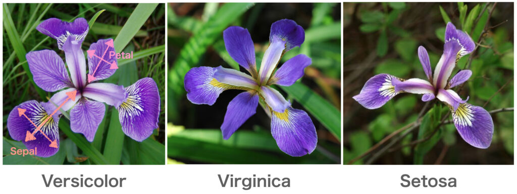
例として用いるデータはirisデータセットを使用します。 irisデータセットは3種類の品種: Versicolour, Virginica, Setosa の花弁(petal)とガク(sepal)の長さで構成されています。
scikit-learnライブラリを用いてirisデータセットを読み込んでみましょう。
import numpy as np
import pandas as pd
from sklearn.datasets import load_iris

iris = load_iris()  # irisデータセットの読み込み
df_iris = pd.DataFrame(iris.data, columns=iris.feature_names)
df_iris['class'] = iris.target
df_iris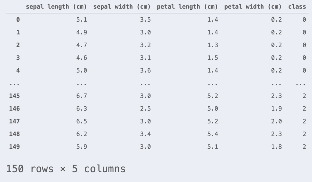
今回はロジスティック回帰の2値分類をおこないます。class = 0, 1 のデータだけに注目します。また、簡単のために特徴量は petal length, petal width の2つとします。
df_iris = df_iris[df_iris['class'] != 2]  # class = 0, 1のデータのみを取得
df_iris = df_iris[['petal length (cm)', 'petal width (cm)', 'class']]
X = df_iris.iloc[:, :-1].values
y = df_iris.iloc[:, -1].values
また、データセットの平均値0, 標準偏差1となるように標準化をおこないます。
from sklearn.preprocessing import StandardScaler

# 標準化のインスタンスを生成(平均=0, 標準偏差=1 に変換)
sc = StandardScaler()
X_std = sc.fit_transform(X)
モデルの汎化性能を評価するために、データセットを訓練データセットとテストデータセットに分割します。ここでは訓練データ80%, テストデータ20%の割合で分割しました。
from sklearn.model_selection import train_test_split

X_train, X_test, y_train, y_test = train_test_split(X_std, y, test_size=0.2, random_state=1, stratify=y)
また、プロットクラスもここで定義しておきます。
# 分類境界のプロットクラスを定義
import matplotlib.pyplot as plt
from matplotlib.colors import ListedColormap

class DecisionPlotter:
    def __init__(self, X, y, classifier, test_idx=None):
        self.X = X
        self.y = y
        self.classifier = classifier
        self.test_idx = test_idx
        self.colors = ['#de3838', '#007bc3', '#ffd12a']
        self.markers = ['o', 'x', ',']
        self.labels = ['setosa', 'versicolor', 'virginica']

    def plot(self):
        cmap = ListedColormap(self.colors[:len(np.unique(self.y))])
        # グリットポイントの生成
        xx1, xx2 = np.meshgrid(
            np.arange(self.X[:,0].min()-1, self.X[:,0].max()+1, 0.01),
            np.arange(self.X[:,1].min()-1, self.X[:,1].max()+1, 0.01))
        # 各meshgridの予測値を求める
        Z = self.classifier.predict(np.array([xx1.ravel(), xx2.ravel()]).T)
        Z = Z.reshape(xx1.shape)
        # 等高線のプロット
        plt.contourf(xx1, xx2, Z, alpha=0.2, cmap=cmap)
        plt.xlim(xx1.min(), xx1.max())
        plt.ylim(xx2.min(), xx2.max())
        # classごとにデータ点をプロット
        for idx, cl, in enumerate(np.unique(self.y)):
            plt.scatter(
                x=self.X[self.y==cl, 0], y=self.X[self.y==cl, 1],
                alpha=0.8,
                c=self.colors[idx],
                marker=self.markers[idx],
                label=self.labels[idx])
        # テストデータの強調
        if self.test_idx is not None:
            X_test, y_test = self.X[self.test_idx, :], self.y[self.test_idx]
            plt.scatter(
                X_test[:, 0], X_test[:, 1],
                alpha=0.9,
                c='None',
                edgecolor='gray',
                marker='o',
                s=100,
                label='test set')
        plt.legend()
\begin{align*}
\newcommand{\mat}[1]{\begin{pmatrix} #1 \end{pmatrix}}
\newcommand{\f}[2]{\frac{#1}{#2}}
\newcommand{\pd}[2]{\frac{\partial #1}{\partial #2}}
\newcommand{\d}[2]{\frac{{\rm d}#1}{{\rm d}#2}}
\newcommand{\T}{\mathsf{T}}
\newcommand{\dis}{\displaystyle}
\newcommand{\eq}[1]{{\rm Eq}(\ref{#1})}
\newcommand{\n}{\notag\\}
\newcommand{\t}{\ \ \ \ }
\newcommand{\argmax}{\mathop{\rm arg\, max}\limits}
\newcommand{\argmin}{\mathop{\rm arg\, min}\limits}
\def\l<#1>{\left\langle #1 \right\rangle}
\def\us#1_#2{\underset{#2}{#1}}
\def\os#1^#2{\overset{#2}{#1}}
\newcommand{\case}[1]{\{ \begin{array}{ll} #1 \end{array} \right.}
\newcommand{\s}[1]{{\scriptstyle #1}}
\end{align*}
フルスクラッチで実装
ロジスティック回帰をフルスクラッチで実装します。前回の結果から、ロジスティック回帰の損失関数 $J$ は次式でした。
\begin{align}
J =\, – \sum_{i=1}^n \{ y^{(i)}\log p^{(i)} + (1 – y^{(i)}) \log (1-p^{(i)}) \}.
\end{align}
そして、最急降下法によるパラメータ $\bm{w}$ の更新規則は以下でした。
\begin{align*}
\bm{w}^{[t+1]} = \bm{w}^{[t]} – \eta\pd{J(\bm{w})}{\bm{w}}.
\end{align*}
観測された $n$ 個の $p$ 次元データを
\begin{align*}
X = \mat{1 & x_1^{(1)} & x_2^{(1)} & \cdots & x_p^{(1)} \\ 1 & x_1^{(2)} & x_2^{(2)} &\cdots & x_p^{(2)} \\ \vdots & \vdots & \vdots & \ddots & \vdots \\ 1 & x_1^{(n)} & x_2^{(n)} &\cdots & x_p^{(n)}\\}.
\end{align*}
と表し、$n$ 個の目的変数 $y^{(i)}$ 、反応確率 $p^{(i)}$ をそれぞれ
\begin{align*}
\bm{y} = \(y^{(1)} , y^{(2)} , \dots , y^{(n)}\)^\T, \t \bm{p} = \(p^{(1)} , p^{(2)} , \dots , p^{(n)}\)^\T
\end{align*}
とすると、$\pd{J(\bm{w})}{\bm{w}}$ は下記と表記できるのでした。
\begin{align}
\pd{J(\bm{w})}{\bm{w}} =\large X^\T(\bm{p}\, -\, \bm{y}).
\end{align}
以上をふまえてロジスティック回帰を実装します。
class LogisticRegression:
    """ロジスティック回帰実行クラス

    Attributes
    ----------
    eta : float
        学習率
    epoch : int
        エポック数
    random_state : int
        乱数シード
    is_trained : bool
        学習完了フラグ
    num_samples : int
        学習データのサンプル数
    num_features : int
        特徴量の数
    w : NDArray[float]
        パラメータベクトル
    costs : NDArray[float]
        各エポックでの損失関数の値の履歴

    Methods
    -------
    fit -> None
        学習データについてパラメータベクトルを適合させる
    predict -> NDArray[int]
        予測値を返却する
    """
    def __init__(self, eta=0.01, n_iter=50, random_state=42):
        self.eta = eta
        self.n_iter = n_iter
        self.random_state = random_state
        self.is_trained = False

    def fit(self, X, y):
        """
        学習データについてパラメータベクトルを適合させる

        Parameters
        ----------
        X : NDArray[NDArray[float]]
            学習データ: (num_samples, num_features)の行列
        y : NDArray[int]
            学習データの教師ラベル: (num_features, )のndarray
        """
        self.num_samples = X.shape[0]  # サンプル数
        self.num_features = X.shape[1]  # 特徴量の数
        # 乱数生成器
        rgen = np.random.RandomState(self.random_state)
        # 正規乱数を用いてパラメータベクトルを初期化
        self.w = rgen.normal(loc=0.0, scale=0.01, size=1+self.num_features)
        self.costs = []  # 各エポックでの損失関数の値を格納する配列
        # パラメータベクトルの更新
        for _ in range(self.n_iter):
            net_input = self._net_input(X)
            output = self._activation(net_input)
            # 式(2)
            self.w[1:] += self.eta * X.T @ (y - output)
            self.w[0] += self.eta * (y - output).sum()
            # 損失関数: 式(1)
            cost = (-y @ np.log(output)) - ((1-y) @ np.log(1-output))
            self.costs.append(cost)
        # 学習完了のフラグを立てる
        self.is_trained = True

    def predict(self, X):
        """
        予測値を返却する

        Parameters
        ----------
        X : NDArray[NDArray[float]]
            予測するデータ: (any, num_features)の行列

        Returens
        -----------
        NDArray[int]
            0 or 1 (any, )のndarray
        """
        if not self.is_trained:
            raise Exception('This model is not trained.')
        return np.where(self._activation(self._net_input(X)) >= 0.5, 1, 0)

    def _net_input(self, X):
        """
        データとパラメータベクトルの内積を計算する

        Parameters
        --------------
        X : NDArray[NDArray[float]]
            データ: (any, num_features)の行列

        Returns
        -------
        NDArray[float]
            データとパラメータベクトルの内積の値
        """
        return X @ self.w[1:] + self.w[0]

    def _activation(self, z):
        """
        活性化関数(シグモイド関数)

        Parameters
        ----------
        z : NDArray[float]
            (any, )のndarray

        Returns
        -------
        NDArray[float]
            各成分に活性化関数を適応した (any, )のndarray
        """
        return 1 / (1 + np.exp(-np.clip(z, -250, 250)))
それでは、irisデータセットを用いて実装を確認してみます。
# ロジスティック回帰モデルの学習
lr = LogisticRegression(eta=0.5, n_iter=1000, random_state=42)
lr.fit(X_train, y_train)

# 訓練データとテストデータを結合
X_comb = np.vstack((X_train, X_test))
y_comb = np.hstack((y_train, y_test))
# プロット
dp = DecisionPlotter(X=X_comb, y=y_comb, classifier=lr, test_idx=range(len(y_train), len(y_comb)))
dp.plot()
plt.xlabel('petal length [standardized]')
plt.ylabel('petal width [standardized]')
plt.show()
このように決定曲線がプロットできました。
scikit-learnを用いた実装
scikit-learn を用いれば、非常に簡単にロジスティック回帰を実行することができます。
from sklearn.linear_model import LogisticRegression

# ロジスティック回帰のインスタンスを作成
lr = LogisticRegression(C=1, random_state=42, solver='lbfgs')
# モデルの学習
lr.fit(X_train, y_train)
irisデータセットを用いて実装を確認してみます。
# 訓練データとテストデータを結合
X_comb = np.vstack((X_train, X_test))
y_comb = np.hstack((y_train, y_test))
# プロット
dp = DecisionPlotter(X=X_comb, y=y_comb, classifier=lr, test_idx=range(len(y_train), len(y_comb)))
dp.plot()
plt.xlabel('petal length [standardized]')
plt.ylabel('petal width [standardized]')
plt.show()
scikit-learnでもこのように決定曲線がプロットできました。
以上のコードはこちら▼で試すことができます。