Introduction
Support Vector Machine (SVM) is a type of supervised machine learning algorithm for pattern recognition.
Based on the idea of “maximizing the margin,” it has high generalization ability and the advantage of not having the problem of convergence to local minima, making it an excellent algorithm for binary classification.
There is “hard margin,” which assumes linearly separable data, and “soft margin,” which assumes linearly inseparable data and allows for some misclassification. This article explains the theory of hard margin Support Vector Machines.
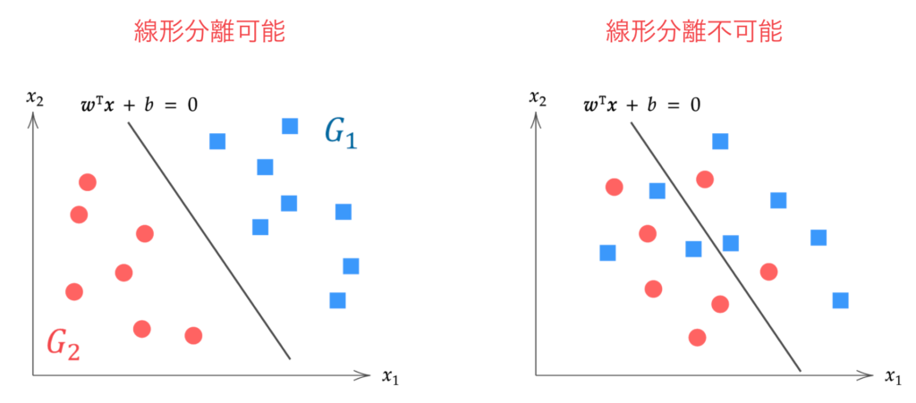
Linearly inseparable: When data cannot be separated by any hyperplane (Right)
▼Theory of Soft Margin SVM is here

\begin{align*}
\newcommand{\mat}[1]{\begin{pmatrix} #1 \end{pmatrix}}
\newcommand{\f}[2]{\frac{#1}{#2}}
\newcommand{\pd}[2]{\frac{\partial #1}{\partial #2}}
\newcommand{\d}[2]{\frac{{\rm d}#1}{{\rm d}#2}}
\newcommand{\T}{\mathsf{T}}
\newcommand{\dis}{\displaystyle}
\newcommand{\eq}[1]{{\rm Eq}(\ref{#1})}
\newcommand{\n}{\notag\\}
\newcommand{\t}{\ \ \ \ }
\newcommand{\tt}{\t\t\t\t}
\newcommand{\argmax}{\mathop{\rm arg\, max}\limits}
\newcommand{\argmin}{\mathop{\rm arg\, min}\limits}
\def\l<#1>{\left\langle #1 \right\rangle}
\def\us#1_#2{\underset{#2}{#1}}
\def\os#1^#2{\overset{#2}{#1}}
\newcommand{\case}[1]{\{ \begin{array}{ll} #1 \end{array} \right.}
\newcommand{\s}[1]{{\scriptstyle #1}}
\newcommand{\c}[2]{\textcolor{#1}{#2}}
\newcommand{\ub}[2]{\underbrace{#1}_{#2}}
\end{align*}
Hard Margin SVM
The goal of the hard margin Support Vector Machine is to find the “optimal” hyperplane $\bm{w}^\T \bm{x} + b = 0$ that completely separates the data of two classes.
Here, $\bm{x}$ and $\bm{w}$ are a $p$-dimensional data vector and a $p$-dimensional parameter vector, respectively.
\begin{align*}
\bm{x} = \mat{x_1 \\ x_2 \\ \vdots \\ x_p},\t \bm{w} = \mat{w_1 \\ w_2 \\ \vdots \\ w_p}.
\end{align*}
Although any number of hyperplanes can be drawn to completely separate the two classes of data, the “optimal” hyperplane is the separating hyperplane that maximizes the margin.
Here, the distance between the separating hyperplane and the data closest to that separating hyperplane is called the margin.
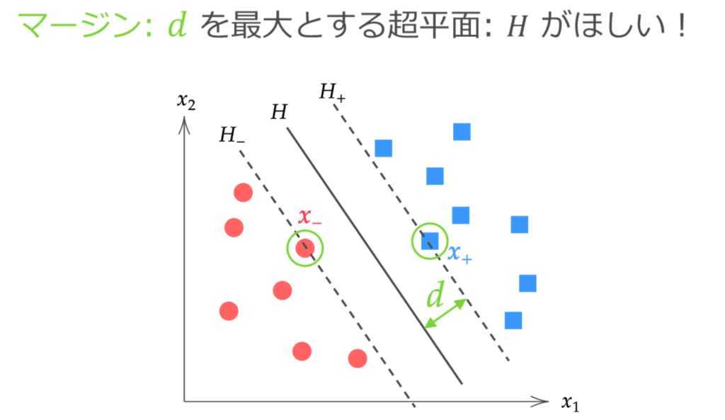
The margin $d$ is obtained as follows from the calculation of the distance between a point and a hyperplane.
\begin{align*}
d = \f{|\bm{w}^\T\bm{x}_{+} + b|}{\|\bm{w}\|} = \f{|\bm{w}^\T\bm{x}_{-} + b|}{\|\bm{w}\|}.
\end{align*}

When finding the optimal separating hyperplane $H: \hat{\bm{w}}^\T \bm{x} + \hat{b} = 0$, we use the fact that no data exists between the hyperplanes $H_{+}$ and $H_{-}$, as shown in the figure above.
In other words, the problem of the hard margin Support Vector Machine can be reduced to the problem of “finding $\bm{w}, b$ that maximize the margin $d$, under the condition that the distance of all data from the hyperplane is at least $d$.”
\{ \hat{\bm{w}}, \hat{b} \} = \argmax_{\bm{w}, b} d(\bm{w}, b)\t {\rm subject\ to}\ \f{|\bm{w}^\T \bm{x}^{(i)} + b|}{\| \bm{w} \|} \geq d \n
i = 1, 2, \dots, n.
\label{eq:cond}
\end{align}
However, the above equation uses absolute values in the constraint condition, which is a bit difficult to handle. Since we are assuming linearly separable data this time, let’s introduce a label variable $y^{(i)}$ to remove the absolute values.
\begin{align*}
y^{(i)} = \case{1 & (\bm{x}^{(i)} \in G_1) \\ -1 & (\bm{x}^{(i)} \in G_2)}
\end{align*}
The label variable $y^{(i)}$ is a variable that takes $y=1$ when the data $\bm{x}^{(i)}$ belongs to group $G_1$ (blue) and $y=-1$ when the data belongs to group $G_2$ (red), as shown in the figure below.
Then, the following holds for the group to which the data $\bm{x}^{(i)}$ belongs.
\begin{align*}
\bm{x}^{(i)} \in G_1 \Leftrightarrow \bm{w}^\T \bm{x}^{(i)} + b > 0 \n
\bm{x}^{(i)} \in G_2 \Leftrightarrow \bm{w}^\T \bm{x}^{(i)} + b < 0
\end{align*}

Therefore, for any data,
|\bm{w}^\T\bm{x}^{(i)} + b| = y^{(i)} (\bm{w}^\T \bm{x}^{(i)} + b) > 0, \t (i=1, 2, \dots, n)
\end{align*}
holds true. Thus, $\eq{eq:cond}$ can be transformed into a form without absolute values as follows.
\{ \hat{\bm{w}}, \hat{b} \} = \argmax_{\bm{w}, b} d(\bm{w}, b)\t {\rm subject\ to}\ \f{y^{(i)}(\bm{w}^\T \bm{x}^{(i)} + b)}{\| \bm{w} \|} \geq d \n
i = 1, 2, \dots, n.
\label{eq:cond2}
\end{align}
Now, let’s simplify the above equation a bit more.
Even if we multiply the condition part of the above equation by a constant, such that $\bm{w} \to c \bm{w},\ b \to c b$,
\f{y^{(i)}(c\bm{w}^\T \bm{x}^{(i)} + cb)}{c\| \bm{w} \|} &= \f{cy^{(i)}(\bm{w}^\T \bm{x}^{(i)} + b)}{c\| \bm{w} \|} \n
&= \f{y^{(i)}(\bm{w}^\T \bm{x}^{(i)} + b)}{\| \bm{w} \|} \n
\end{align*}
it becomes as follows, so it is invariant to scaling by an arbitrary constant for $\bm{w}, b$.
Therefore, by transforming the condition part,
\begin{align*}
&\f{y^{(i)}(\bm{w}^\T \bm{x}^{(i)} + b)}{\| \bm{w} \|} \geq d \n
\n
&\downarrow \textstyle\t \s{\text{Divide both sides by } d} \n
\n
&y^{(i)} \bigg( \underbrace{\f{1}{d \| \bm{w} \|} \bm{w}^\T}_{=\bm{w}^{*\T}} \bm{x}^{(i)} + \underbrace{\f{1}{d \| \bm{w} \|} b}_{=b^*} \bigg) \geq 1 \n
\n
&\downarrow \textstyle\t \s{\text{Let } \bm{w}^{*\T} = \f{1}{d \| \bm{w} \|} \bm{w}^\T,\ b^* = \f{1}{d \| \bm{w} \|} b} \n
\n
&y^{(i)} \( \bm{w}^{*\T} \bm{x}^{(i)} + b^* \) \geq 1
\end{align*}
we can see that it is acceptable to scale it as such.
Here, the data $\bm{x}^{(i)}$ for which the equality holds in $y^{(i)} \( \bm{w}^{*\T} \bm{x}^{(i)} + b^* \) \geq 1$ is the data closest to the separating hyperplane, that is, the support vectors $\bm{x}_{+}, \bm{x}_{-}$.
Therefore, the scaled margin $d^*$ is,
d^* &= \f{y_{+} (\bm{w}^{*\T}\c{myblue}{\bm{x}_{+}} + b^* ) }{\| \bm{w}^* \|} = \f{y_{-} (\bm{w}^{*\T}\c{myred}{\bm{x}_{-}} + b^* ) }{\| \bm{w}^* \|} \n
&= \f{1}{\| \bm{w}^* \|}
\end{align*}
as shown.
Thus, $\eq{eq:cond2}$ can be expressed as follows.
\{ \hat{\bm{w}}, \hat{b} \} = \argmax_{\bm{w}^*, b^*} \f{1}{\| \bm{w}^* \|} \t {\rm subject\ to}\ y^{(i)} \( \bm{w}^{*\T} \bm{x}^{(i)} + b^* \) \geq 1 \n
i = 1, 2, \dots, n.
\end{align*}
$\bm{w}^*, b^*$ that maximize $1/ \| \bm{w}^* \|$ are equivalent to $\bm{w}^*, b^*$ that minimize $\| \bm{w}^* \|^2$. From now on, we will denote $\bm{w}^*, b^*$ as $\bm{w}, b$ again, and the following can be stated.
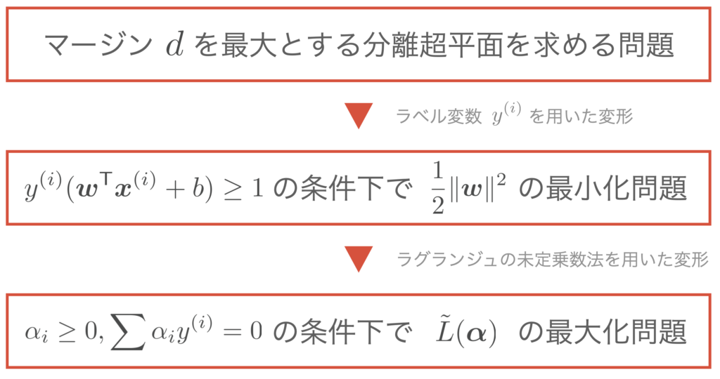
The problem of finding the hyperplane that maximizes the margin can be reduced to the problem of finding the following.
\{ \hat{\bm{w}}, \hat{b} \} = \argmin_{\bm{w}, b} \f{1}{2}\|\bm{w}\|^2 \t {\rm subject\ to}\ y^{(i)} \( \bm{w}^{\T} \bm{x}^{(i)} + b \) \geq 1 \n
i = 1, 2, \dots, n.
\end{align*}
(Here, 1/2 is attached to $\|\bm{w}\|$ to tidy up the equation after differentiation, and it is squared to bring it into the form of a quadratic programming problem)
Transformation using the Method of Lagrange Multipliers
We solve the constrained optimization problem using the method of Lagrange multipliers. Since the constraints are inequalities in this case, the KKT conditions can be applied.
▼ The KKT conditions are explained in this article.

Since there are $n$ constraints corresponding to the number of data points, we define the Lagrangian function $L$ using Lagrange multipliers $\alpha_1, \alpha_2, \dots, \alpha_n$ as follows.
L(\bm{w}, b, \alpha_1, \dots, \alpha_n) \equiv \f{1}{2}\|\bm{w}\|^2 – \sum_{i=1}^n \alpha_i \{ y^{(i)} (\bm{w}^\T \bm{x}^{(i)} + b) – 1 \}.
\end{align*}
Then, at the optimal solution for $\bm{w}$, the following equations hold from the KKT conditions.
\case{
& \dis \pd{L(\bm{w}, b, \alpha_1, \dots, \alpha_n)}{\bm{w}} = \bm{0}, & (☆1) \n
& \dis \pd{L(\bm{w}, b, \alpha_1, \dots, \alpha_n)}{b} = 0, & (☆2) \n
&\alpha_i \geq 0, & (☆3) \n
&\alpha_i = 0,\ \s{\text{or}}\ \ y^{(i)}(\bm{w}^\T \bm{x}^{(i)} + b) – 1 = 0. & (☆4)
}
\end{align*}
From equations (☆1) and (☆2), respectively,
(☆1) &= \pd{L(\bm{w}, b, \alpha_1, \dots, \alpha_n)}{\bm{w}} \n
&= \pd{}{\bm{w}} \( \f{1}{2}\|\bm{w}\|^2 – \sum_{i=1}^n \alpha_i \{ y^{(i)} (\bm{w}^\T \bm{x}^{(i)} + b) – 1 \} \) \n
&= \f{1}{2}\pd{}{\bm{w}}\|\bm{w}\|^2 – \sum_{i=1}^n \alpha_i \pd{}{\bm{w}} \{ y^{(i)} ( \bm{w}^\T \bm{x}^{(i)} + b) – 1 \} \n
&= \bm{w}\, – \sum_{i=1}^n \alpha_iy^{(i)} \bm{x}^{(i)} = \bm{0} \n
& \t\t\t\t \therefore \bm{w} = \sum_{i=1}^n \alpha_i y^{(i)}\bm{x}^{(i)}.
\label{eq:lag1}
\end{align}
(☆2) &= \pd{L(\bm{w}, b, \alpha_1, \dots, \alpha_n)}{b} \n
&= \pd{}{b} \( \f{1}{2}\|\bm{w}\|^2 – \sum_{i=1}^n \alpha_i \{ y^{(i)} (\bm{w}^\T \bm{x}^{(i)} + b) – 1 \} \) \n
&= -\sum_{i=1}^n \alpha_i y^{(i)} = 0 \n
& \t\t\t\t \therefore \sum_{i=1}^n \alpha_i y^{(i)} = 0.
\label{eq:lag2}
\end{align}
are obtained. Now, by substituting $\eq{eq:lag1},(\ref{eq:lag2})$ into $L(\bm{w}, b, \alpha_1, \dots, \alpha_n)$ to eliminate $\bm{w}, b$,
L(\bm{w}, b, \alpha_1, \dots, \alpha_n) &\equiv \f{1}{2}\|\bm{w}\|^2 – \sum_{i=1}^n \alpha_i \{ y^{(i)} (\bm{w}^\T \bm{x}^{(i)} + b) – 1 \} \n
&= \f{1}{2}\|\bm{w}\|^2 – \ub{\sum_{i=1}^n \alpha_i y^{(i)} \bm{x}^{(i) \T}}{=\bm{w}^\T} \bm{w} \, – \ub{\sum_{i=1}^n\alpha_i y^{(i)}}{=0} b + \sum_{i=1}^n \alpha_i \n
&= \f{1}{2}\|\bm{w}\|^2 -\| \bm{w} \|^2 + \sum_{i=1}^n \alpha_i \n
&= \sum_{i=1}^n \alpha_i -\f{1}{2}\|\bm{w}\|^2 \n
&= \sum_{i=1}^n \alpha_i – \frac{1}{2} \sum_{i=1}^{n} \sum_{j=1}^{n} \alpha_{i} \alpha_{j} y^{(i)} y^{(j)}\boldsymbol{x}^{(i)\T}\boldsymbol{x}^{(j)} \n
&\equiv \tilde{L}(\alpha_1, \dots, \alpha_n)
\label{eq:L_tilde}
\end{align}
the Lagrangian function $L$ can be transformed into a function $\tilde{L}(\alpha_1, \dots, \alpha_n)$ of only $\alpha$, as shown above. Also, from its form, it can be seen that $\tilde{L}$ is a concave function (convex upward) with respect to $\alpha$.
From the above discussion, instead of the minimization problem of $\f{1}{2} \|\bm{w} \|^2$, if we find the optimal solution $\hat{\bm{\alpha}}$ from the maximization problem of $\tilde{L}(\bm{\alpha})$, we can obtain the original solution $\hat{\bm{w}}$ (this discussion is called the dual problem).
The problem of finding the hyperplane that maximizes the margin can be reduced to the problem of finding the following.
\hat{\bm{\alpha}} &= \argmax_{\bm{\alpha}} \tilde{L}(\bm{\alpha}) \n
&= \argmax_{\bm{\alpha}} \{ \sum_{i=1}^n \alpha_i – \frac{1}{2} \sum_{i=1}^{n} \sum_{j=1}^{n} \alpha_{i} \alpha_{j} y^{(i)} y^{(j)}\boldsymbol{x}^{(i)\T}\boldsymbol{x}^{(j)} \} \n
& \tt {\rm subject\ to}\ \alpha_i \geq 0, \sum_{i=1}^n \alpha_i y^{(i)} = 0,\ (i = 1, 2, \dots, n).
\end{align*}
Summarizing the discussion so far, it becomes as follows.
Estimation of $\hat{\bm{\alpha}}$ using Gradient Descent
Here, we use the gradient descent method to find the optimal solution $\hat{\bm{\alpha}}$. In the gradient descent method, we randomly set the initial value of the parameter $\bm{\alpha}^{[0]}$, and since it is a maximization problem, we update the parameters in the ascending direction, which is the direction of the gradient vector, as shown below.
\begin{align}
\bm{\alpha}^{[t+1]} = \bm{\alpha}^{[t]} + \eta \pd{\tilde{L}(\bm{\alpha})}{\bm{\alpha}}.
\label{eq:kouka}
\end{align}
To perform gradient descent, let’s calculate the value of the gradient vector $\pd{\tilde{L}(\bm{\alpha})}{\bm{\alpha}}$.
As preparation for the calculation, first rewrite $\eq{eq:L_tilde}$ using vector notation.
Let us represent the observed $n$ pieces of $p$-dimensional data using a matrix as follows.
\us X_{[n \times p]} = \mat{x_1^{(1)} & x_2^{(1)} & \cdots & x_p^{(1)} \\
x_1^{(2)} & x_2^{(2)} & \cdots & x_p^{(2)} \\
\vdots & \vdots & \ddots & \vdots \\
x_1^{(n)} & x_2^{(2)} & \cdots & x_p^{(n)}}
=
\mat{ – & \bm{x}^{(1)\T} & – \\
– & \bm{x}^{(2)\T} & – \\
& \vdots & \\
– & \bm{x}^{(n)\T} & – \\}.
\end{align*}
Also, let us represent the $n$ label variables $y^{(i)}$ and Lagrange multipliers $\alpha_i$ using column vectors as follows, respectively.
\begin{align*}
\us \bm{y}_{[n \times 1]} = \mat{y^{(1)} \\ y^{(2)} \\ \vdots \\ y^{(n)}},
\t
\us \bm{\alpha}_{[n \times 1]} = \mat{\alpha_1 \\ \alpha_2 \\ \vdots \\ \alpha_n}.
\end{align*}
Here, let’s define a new matrix $H$ as
\begin{align*}
\us H_{[n \times n]} \equiv \us \bm{y}_{[n \times 1]} \us \bm{y}^{\T}_{[1 \times n]} \odot \us X_{[n \times p]} \us X^{\T}_{[p \times n]}
\end{align*}
(where $\odot$ is the Hadamard product).
In other words, the components of the above matrix are $(H)_{ij} = y^{(i)}y^{(j)} \bm{x}^{(i)\T} \bm{x}^{(j)}$, and $H$ is a symmetric matrix.
Then, $\eq{eq:L_tilde}$ becomes
\tilde{L}(\bm{\alpha}) &\equiv \sum_{i=1}^n \alpha_i – \frac{1}{2} \sum_{i=1}^{n} \sum_{j=1}^{n} \alpha_{i} \alpha_{j} y^{(i)} y^{(j)}\boldsymbol{x}^{(i)\T}\boldsymbol{x}^{(j)} \n
&= \sum_{i=1}^n \alpha_i – \frac{1}{2} \sum_{i=1}^{n} \sum_{j=1}^{n} \alpha_{i} \alpha_{j} (H)_{ij} \n
&= \| \bm{\alpha} \| -\f{1}{2} \bm{\alpha}^\T H \bm{\alpha}
\end{align*}
and can be expressed using vectors.
Therefore, the gradient vector $\pd{\tilde{L}(\bm{\alpha})}{\bm{\alpha}}$ can be calculated as follows using the vector differentiation formulas.
\begin{align*}
\pd{\tilde{L}(\bm{\alpha})}{\bm{\alpha}} &= \pd{}{\bm{\alpha}} \| \bm{\alpha} \| -\f{1}{2} \pd{}{\bm{\alpha}} \bm{\alpha}^\T H \bm{\alpha} \n
&= \bm{1}\, – H \bm{\alpha}.
\end{align*}
Here, $\bm{1}$ is an $n$-dimensional column vector where all components are 1, $ \bm{1} = (1, 1, \dots, 1)^\T $.

From the above, the update rule $\eq{eq:kouka}$ for the Lagrange multiplier $\bm{\alpha}$ becomes
\begin{align*}
\bm{\alpha}^{[t+1]} = \bm{\alpha}^{[t]} + \eta \( \bm{1}\, – H \bm{\alpha}^{[t]} \)
\end{align*}
as shown.
Calculating the Parameters $\hat{\bm{w}}, \hat{b}$ of the Separating Hyperplane
The goal of the hard margin SVM is to find the separating hyperplane that maximizes the margin, in other words, to find the parameters $\hat{\bm{w}}, \hat{b}$ of the separating hyperplane.
Now, if we can calculate the optimal solution of the Lagrange multipliers $\hat{\bm{\alpha}}$ using the gradient descent method, we can subsequently find $\hat{\bm{w}}, \hat{b}$.
Finding $\hat{\bm{w}}$
Once the optimal solution of the Lagrange multipliers $\hat{\bm{\alpha}}$ is found, $\hat{\bm{w}}$ can be calculated from $\eq{eq:lag1}$.
\begin{align}
\hat{\bm{w}} = \sum_{i=1}^n \hat{\alpha}_i y^{(i)} \bm{x}^{(i)}.
\label{eq:w}
\end{align}
Now, let’s consider the above equation a bit more. From the KKT condition (☆4), for $\hat{\alpha}_i$ and $\bm{x}^{(i)}$,
\begin{align*}
\hat{\alpha_i} = 0,\ \s{\text{or}}\ \ y^{(i)}(\bm{w}^\T \bm{x}^{(i)} + b) – 1 = 0
\end{align*}
the relationship holds. On the other hand, the data $\bm{x}^{(i)}$
\case{y^{(i)}(\bm{w}^\T \bm{x}^{(i)} + b) – 1 = 0 & (\bm{x}^{(i)} \s{\text{is a support vector}}), \\
y^{(i)}(\bm{w}^\T \bm{x}^{(i)} + b) – 1 > 0 & \rm{(otherwise)}}
\end{align*}
has the relationship, so the following can be said.
\begin{align*}
\case{
\hat{\alpha}_i \neq 0 \Leftrightarrow \bm{x}^{(i)} \s{\text{is a support vector}}, \\
\hat{\alpha}_i = 0 \Leftrightarrow \bm{x}^{(i)} \s{\text{is not a support vector}}. \\
}
\end{align*}
Therefore, in the sum of $\eq{eq:w}$, $\hat{\alpha}_i = 0$ for the indices of data that are not support vectors, so they do not contribute to the summation. In other words, we only need to sum over the support vectors, which saves computational cost.
\begin{align*}
\hat{\bm{w}} = \sum_{\bm{x}^{(i)} \in S} \hat{\alpha}_i y^{(i)} \bm{x}^{(i)}.
\end{align*}
(Here, $S$ is the set of support vectors)
Finding $\hat{b}$
Once $\hat{\bm{w}}$ is found from the above, $\hat{b}$ can be calculated from the relation $y^{(i)}(\hat{\bm{w}}^\T \bm{x}^{(i)} + \hat{b}) – 1 = 0$ when $\bm{x}^{(i)}$ is a support vector.
\begin{align*}
\hat{b} &= \f{1}{y^{(i)}} – \hat{\bm{w}}^\T \bm{x}^{(i)} \n
&= y^{(i)} – \hat{\bm{w}}^\T \bm{x}^{(i)} \t (\because y^{(i)} = 1, -1).
\end{align*}
In this way, $\hat{b}$ can be calculated if there is at least one support vector, but in practice, to reduce error, we calculate the average over all support vectors as follows.
\begin{align*}
\hat{b} = \f{1}{|S|} \sum_{\bm{x}^{(i)} \in S} (y^{(i)} – \hat{\bm{w}}^\T \bm{x}^{(i)}).
\end{align*}
(Here, $|S|$ is the number of support vectors)
From the above, the separating hyperplane can be determined by finding $\hat{\bm{w}}, \hat{b}$.
Implementation of Support Vector Machine is here ▼