Classification Evaluation Indicators: Accuracy, Precision, Recall, F-measure

This article is available in: 日本語

Introduction
Metrics for Classification Problem Evaluation
Calculation of evaluation indicators using scikit-learn

Introduction

After a model (classifier) is trained by machine learning in a classification problem, its performance needs to be evaluated.

This article discusses the following, which are its evaluation indicators

Accuracy
Precision
Recall / True Positive Rate: TPR
False Positive Rate: FPR
F-measure

We also describe how to calculate the above using scikit-learn.

You can try the source code for this article from google colab below.

Google Colaboratory

Metrics for Classification Problem Evaluation

To simplify matters, we will limit our discussion to the two classes of classification problems. Here, we consider classifying data as either + (positive) or – (negative).

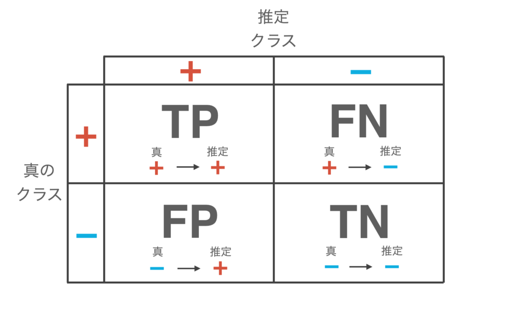
Now, when the classifier is fed test data and allowed to make inferences, the following four patterns arise.

True Positive (TP): Infer + for data whose true class is +.
False Negative (FN): Infer data whose true class is + as –.
False Positive (FP): Infer data with a true class of – as +.
True negative (TN): Infer data with true class – as –.

The results of this classification are summarized in a table as shown below, which is called the confusion matrix. The diagonal components of this table indicate the number of data for which the inference is correct, and the off-diagonal components indicate the number of data for which the inference is incorrect.

These four patterns above define the evaluation indicators for various classifiers.

Accuracy

The accuracy is the proportion of the test data that the classifier correctly infers and is expressed by the following equation

\begin{align*} {\rm accuracy} = \frac{{\rm TP} + {\rm TN}}{{\rm TP} + {\rm FP} + {\rm FN} + {\rm TN}} \end{align*}

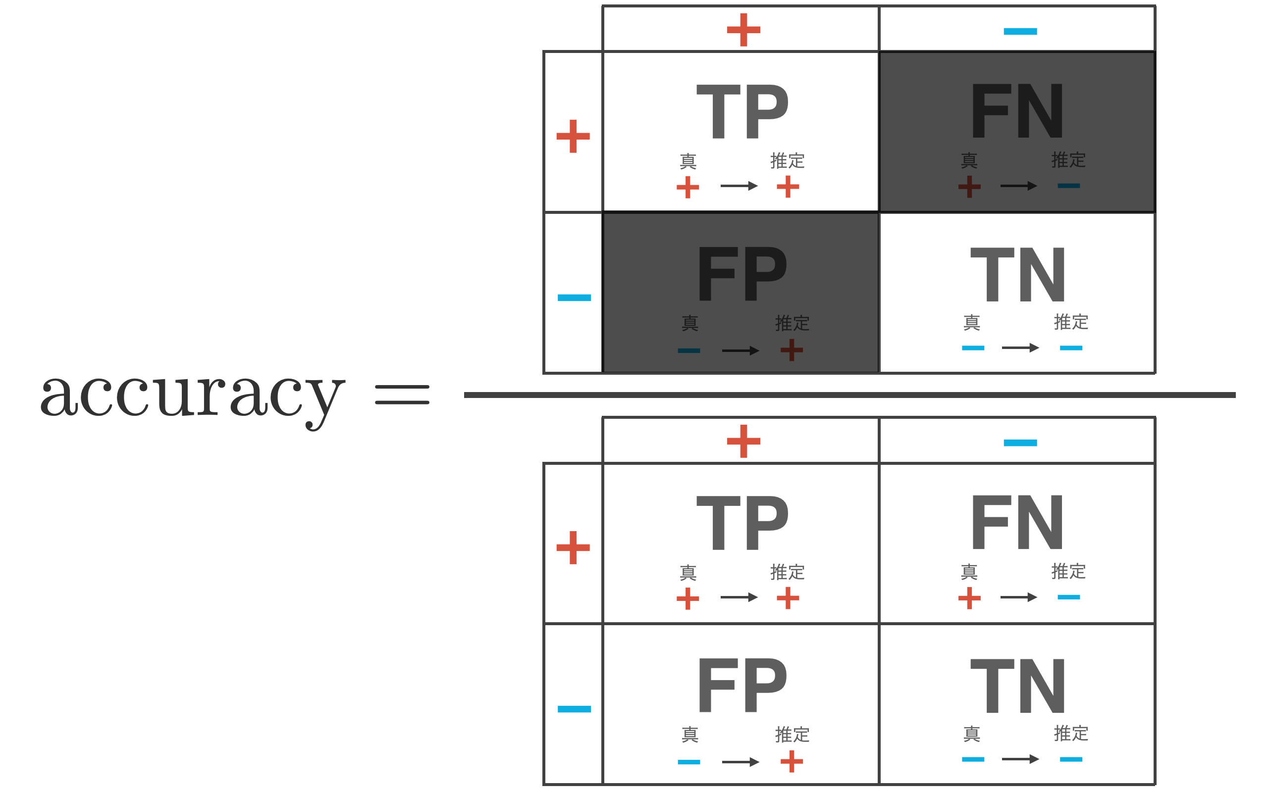
+ (positive) and – (negative), so it is an expression for the percentage of ${\rm TP} + {\rm TN}$ cases out of the total number of data ${\rm TP} + {\rm FP} + {\rm FN} + {\rm TN}$.

Now, a problem arises when evaluating classifier performance based solely on this percentage of correct answers.

As an example, let’s consider a data set of 100,000 data, of which 99990 are – (negative) and 10 are + (positive).

Suppose a discriminator estimates all data to be – (negative) as shown in the following table.

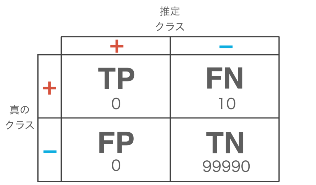
▲If all 100,000 data are estimated to be – (negative)

At this point, we calculate accuracy

\begin{align*} {\rm accuracy} &= \frac{{\rm TP} + {\rm TN}}{{\rm TP} + {\rm FP} + {\rm FN} + {\rm TN}} \\ &= \frac{0 + 99990}{0 + 0 + 10 + 99990} \\ &= 0.9999 = 99.99 \% \end{align*}

The accuracy is so high that it is considered a good classifier even though it has not detected a single + (positive) case.

In other words, it is not sufficient to judge the performance of a classifier by the percentage of correct answers alone, and various indicators have been proposed as follows

Precision

Precision is a measure of how reliable a classifier is when it determines that data is + (positive).

\begin{align*} {\rm precision} = \frac{{\rm TP}}{{\rm TP} + {\rm FP}} \end{align*}

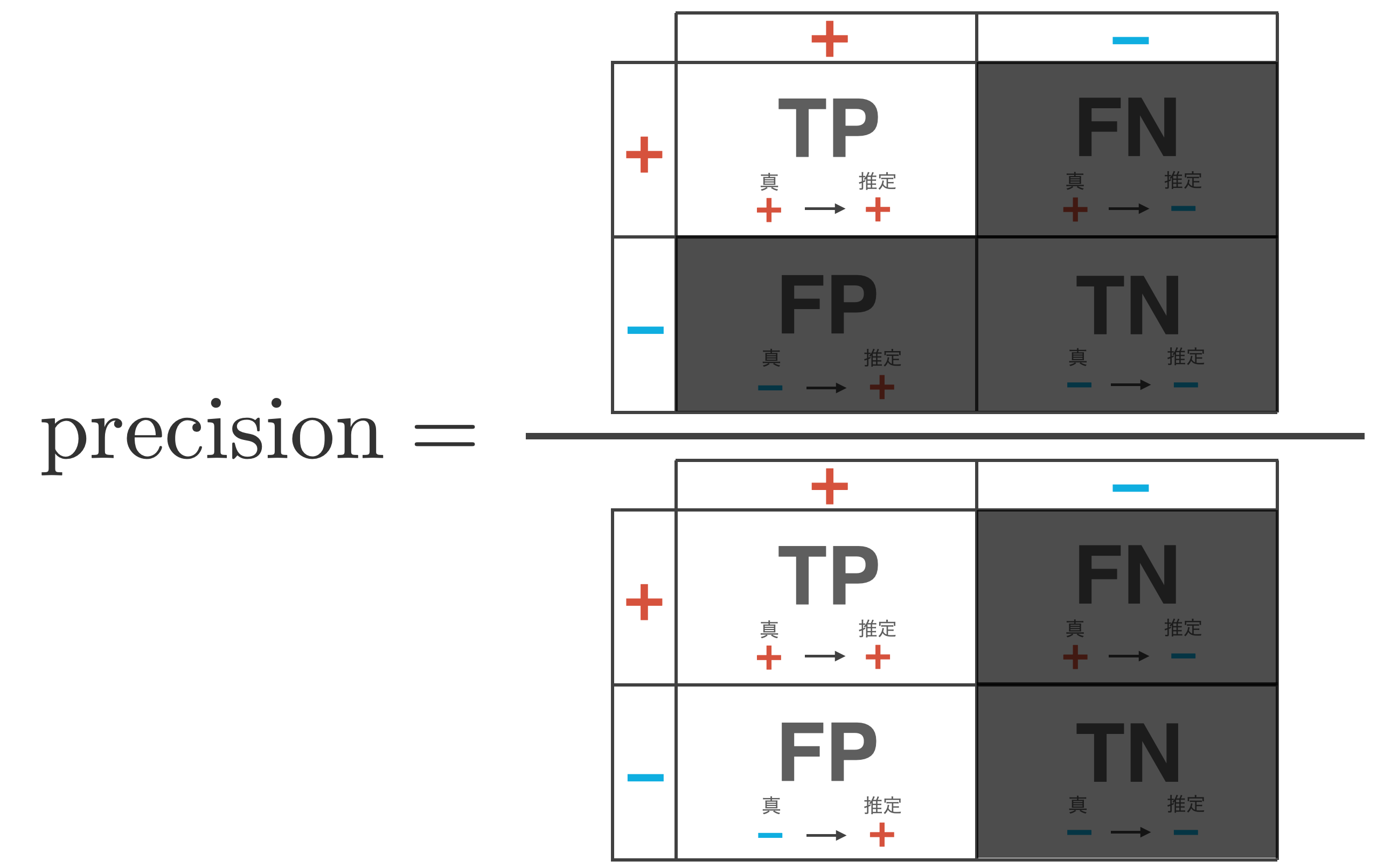
This indicator is mainly used when one wants to increase predictive certainty. However, a classifier that only increases accuracy can be achieved by reducing the number of FPs (the number of cases where – is incorrectly inferred as +), i.e., by using a model that judges + more strictly.

Recall / True Positive Rate: TPR

Recall is a measure of how well the classifier correctly inferred + (positive) out of the total + (positive) data. It is also called the true positive rate (TPR).

\begin{align*} {\rm recall} = \frac{{\rm TP}}{{\rm TP} + {\rm FN}} \end{align*}

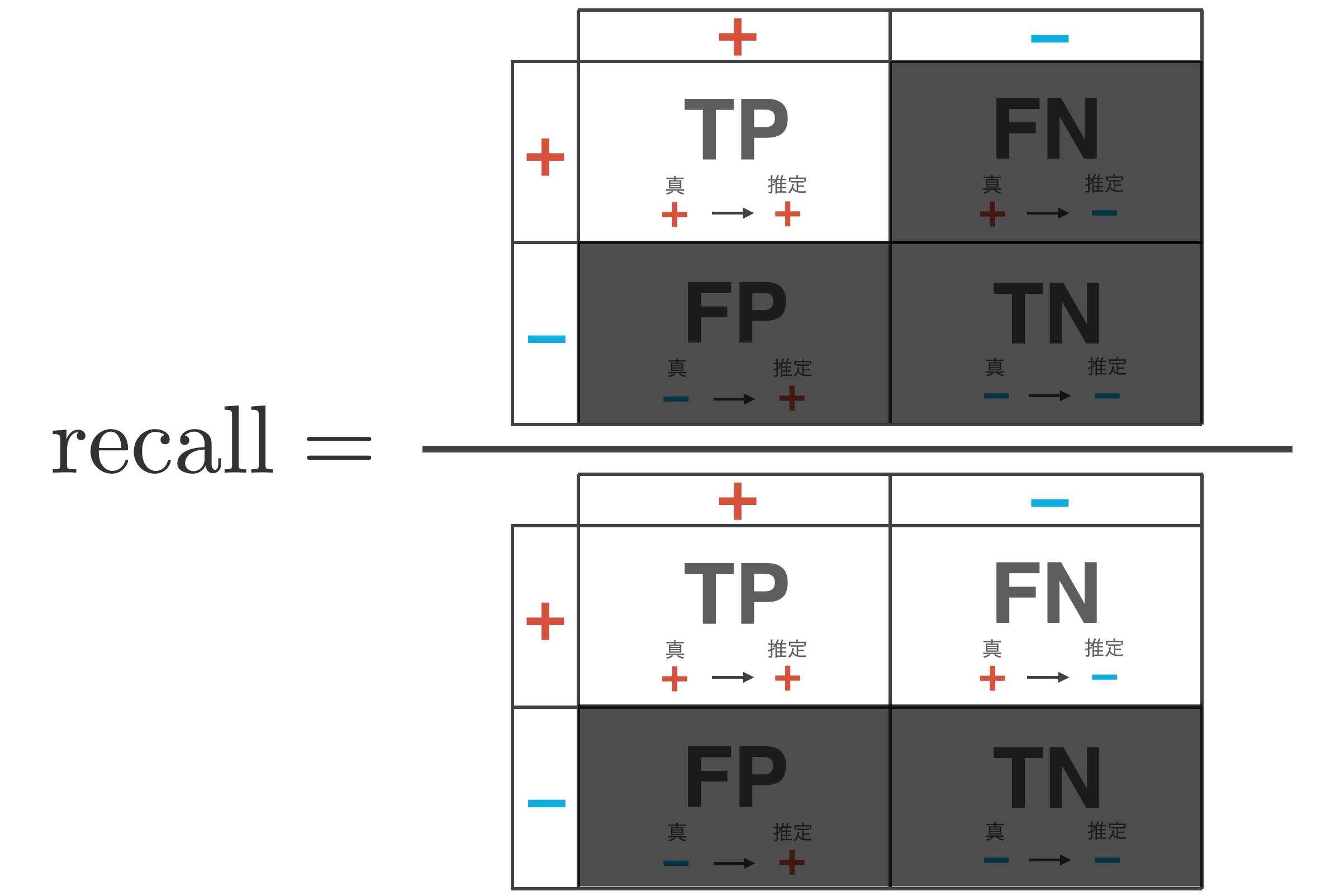
When the importance of reducing FN (the number of cases where + is incorrectly inferred as -) is important, this indicator is used in cases such as cancer diagnosis. However, a classifier that only increases the reproducibility can be achieved with a model that loosely determines +, or in the extreme, a model that determines + for all data.

False Positive Rate: FPR

The false positive rate (FPR) is a measure of how much of the total – (negative) data the classifier incorrectly infers as + (positive).

\begin{align*} {\rm FPR} = \frac{{\rm FP}}{{\rm TN} + {\rm FP}} \end{align*}

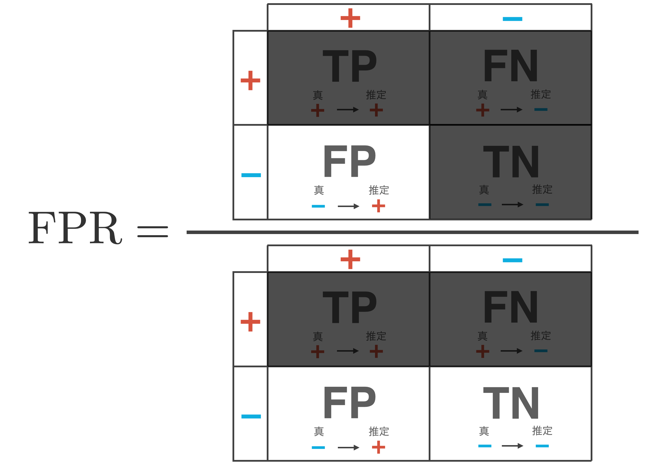
A small value for this indicator is desired. However, a classifier that reduces only the false positive rate can be achieved with a model that judges – for all data.

This FPR and TPR (= recall) are used in the ROC curve.

▼Click here to see the contents of the ROC curve.

https://laid-back-scientist.com/roc-curve

F-measure

There is a trade-off between precision and recall, and these indicators cannot be high at the same time. The reason for the trade-off, as mentioned earlier, is that a classifier that increases only precision is realized with a model that judges “strictly” +, while a classifier that increases only recall is realized with a model that judges “loosely” +.

Now, a model with high precision and recall means a model with low FP and FN, i.e., a high-performance classifier with low off-diagonal components of the confusion matrix = low misclassification. Therefore, we define the F-measure as the harmonic mean of precision and recall.

\begin{align*} F = \frac{2}{\frac{1}{{\rm recall}} + \frac{1}{{\rm precision}}} = 2 \cdot \frac{{\rm precision} \cdot {\rm recall}}{{\rm precision} + {\rm recall}} \end{align*}

Calculation of evaluation indicators using scikit-learn

The above indicators can be easily calculated using scikit-learn.

First, import the necessary libraries and define the data to be handled. The data to be handled in this case is a simple array with 1: positibe, -1: negative.

import numpy as np
import pandas as pd
from sklearn.metrics import confusion_matrix, classification_report
import seaborn as sns
import matplotlib.pyplot as plt

y_true = [-1, -1, -1, -1, -1, 1, 1, 1, 1, 1]
y_pred = [-1, -1, -1, 1, 1, -1, 1, 1, 1, 1]
names = ['positive', 'negative']

First, we generate the confusion matrix, which can be generated in scikit-learn with confusion_matrix.

cm = confusion_matrix(y_true, y_pred, labels=[1, -1])
print(cm)

# Output
[[4 1]
 [2 3]]

To make the output easier to read, let’s display the confusion matrix in seaborn.

cm = pd.DataFrame(data=cm, index=names, columns=names)
sns.heatmap(cm, square=True, cbar=True, annot=True, cmap='Blues')
plt.xlabel('predicted value', fontsize=15)
plt.ylabel('grand truth', fontsize=15)
plt.show()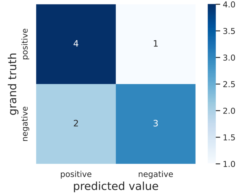

Next, let’s calculate the evaluation index. In scikit-learn, the evaluation indicators described so far can be calculated together using classification_report.

eval_dict = classification_report(y_true, y_pred, output_dict=True, target_names=names)

df = pd.DataFrame(eval_dict)
print(df)

# Output
           positive  negative  accuracy  macro avg  weighted avg
precision  0.750000  0.666667       0.7   0.708333      0.708333
recall     0.600000  0.800000       0.7   0.700000      0.700000
f1-score   0.666667  0.727273       0.7   0.696970      0.696970
support    5.000000  5.000000       0.7  10.000000     10.000000

The first and second columns of the output results show the results of the indicators when positive and negative are used as positive examples, respectively.

Also, macro avg and weighted avg are called macro average and weighted average, respectively.

In this problem set-up, the indicators we want are as follows.

print(f"accuracy: {df['accuracy'][0]:.2f}")
print(f"precision: {df['positive']['precision']:.2f}")
print(f"recall: {df['positive']['recall']:.2f}")
print(f"f1-score: {df['positive']['f1-score']:.2f}")

# Output
accuracy: 0.70
precision: 0.75
recall: 0.60
f1-score: 0.67

You can try the above code in the following google colab

Google Colaboratory