Introduction
When the target variable $y$ is binary data (for example, $y = 0, 1$), this is a type of prediction model for the target variable $x$ that takes real values. As a hypothetical example, suppose we observe $n$ pairs of data where an individual responds to a certain numerical level $x$ with $y=1$, and does not respond with $y=0$.
\begin{align*}
\newcommand{\mat}[1]{\begin{pmatrix} #1 \end{pmatrix}}
\newcommand{\f}[2]{\frac{#1}{#2}}
\newcommand{\pd}[2]{\frac{\partial #1}{\partial #2}}
\newcommand{\d}[2]{\frac{{\rm d}#1}{{\rm d}#2}}
\newcommand{\T}{\mathsf{T}}
\newcommand{\dis}{\displaystyle}
\newcommand{\eq}[1]{{\rm Eq}(\ref{#1})}
\newcommand{\n}{\notag\\}
\newcommand{\t}{\ \ \ \ }
\newcommand{\argmax}{\mathop{\rm arg\, max}\limits}
\newcommand{\argmin}{\mathop{\rm arg\, min}\limits}
\def\l<#1>{\left\langle #1 \right\rangle}
\def\us#1_#2{\underset{#2}{#1}}
\def\os#1^#2{\overset{#2}{#1}}
\newcommand{\case}[1]{\{ \begin{array}{ll} #1 \end{array} \right.}
\newcommand{\s}[1]{{\scriptstyle #1}}
\end{align*}
\(x^{(1)}, y^{(1)}\), \(x^{(2)}, y^{(2)}\), \dots, \(x^{(n)}, y^{(n)}\),\\x^{(i)} \in \mathbb{R}, \t y^{(i)} = \cases{1, & (positive). \\ 0, & (negative).}
\end{align*}
For such binary data, let us consider building a model to estimate the response probability $p$ for a numerical level $x$.

Here, by introducing a random variable $Y$ that represents whether or not a response occurred, the response probability for numerical level $x$ is expressed as $\Pr(Y=1|x) = p$, and the non-response probability is expressed as $\Pr(Y = 0|x)= 1-p$.
To build a model, we must consider the functional form of the response probability $p$. Since $p$ is a probability, its range is $0 \leq p \leq 1$. Also, the factor $x$ that causes the response is a real value: $-\infty < x < \infty$.
The “logistic model” uses the logistic function $\sigma(\cdot)$ as the function that connects $x$ and $p$.
\text{Logistic function: } \sigma(z) \equiv \f{1}{1 + \exp(-z)}.
\end{align*}
That is, in the logistic model, the response probability $p$ is expressed using parameters $w_0, w_1$ as follows.
p = \sigma(w_0 + w_1x) = \f{1}{1 + \exp\[-(w_0 + w_1x)\]}, \\\\(0 \leq p \leq 1), \t (-\infty < x < \infty). \t\t\t
\end{align*}
By estimating the values of parameters $w_0, w_1$ based on the observed $n$ pairs of data, we obtain a model that outputs the probability of responding to any numerical level $x$.
The problem is the parameter estimation method, which we will clarify in the next section.
Estimation of the Logistic Model
While the above description concerned one type of explanatory variable $x$, let us consider more generally the estimation of the probability that the target variable $y$ follows with respect to $p$ explanatory variables.
Now, let the $i$-th data observed for $p$ explanatory variables $x_1, x_2, \dots, x_p$ and target variable $y$ be
\(x_1^{(i)}, x_2^{(i)}, \dots, x_p^{(i)} \), \t y^{(i)} = \cases{1, & (positive) \\ 0, & (negative)}, \\(i = 1, 2, \dots, n).
\end{align*}
Introducing the random variable $Y$ as before, the response probability and non-response probability are respectively
\Pr(Y=1|x_1, \dots x_p) = p,\t \Pr(Y=0|x_1, \dots x_p) = 1-p
\end{align*}
and the relationship between the explanatory variables $x_1, x_2, \dots, x_p$ and the response probability $p$ is connected by
p &= \f{1}{1 + \exp\[-(w_0 + w_1x_1 + w_2x_2 + \cdots + w_px_p)\]} \n&= \f{1}{1 + \exp(-\bm{w}^\T \bm{x})}\label{eq:proj}
\end{align}
Here, $\bm{w} = (w_0, w_1, \dots, w_p)^\T$ and $\bm{x} = (1, x_1, x_2, \dots, x_p)^\T$.
Now let us estimate the value of the parameter vector $\bm{w}$ based on the observed $n$ pairs of data. We will consider estimating the parameters using maximum likelihood estimation.
Now, for the $i$-th data, we have a pair consisting of the random variable $Y^{(i)}$ representing whether or not a response occurred and its realized value $y^{(i)}$. Therefore, letting the true response probability for the $i$-th data be $p^{(i)}$, the response probability and non-response probability are respectively
\Pr(Y^{(i)}=1) = p^{(i)},\t \Pr(Y^{(i)}=0) = 1-p^{(i)}
\end{align*}
In other words, we can see that the probability distribution that the random variable $Y^{(i)}$ follows is the following Bernoulli distribution.
\Pr(Y^{(i)} = y^{(i)}) &= {\rm Bern}(y^{(i)}|p^{(i)}) \\&= (p^{(i)})^{y^{(i)}} (1 – p^{(i)})^{1-y^{(i)}}, \\\\(y^{(i)} = 0, 1),&\t (i=1, 2, \dots, n).
\end{align*}
Therefore, the likelihood function based on $y^{(1)}, y^{(2)}, \dots, y^{(n)}$ is as follows.
L(p^{(1)}, p^{(2)}, \dots, p^{(n)}) &= \prod_{i=1}^n {\rm Bern}(y^{(i)}|p^{(i)}) \n&= \prod_{i=1}^n (p^{(i)})^{y^{(i)}} (1 – p^{(i)})^{1-y^{(i)}}.\label{eq:likelihood}
\end{align}
By substituting $\eq{eq:proj}$ into $\eq{eq:likelihood}$, we see that the likelihood function is a function of the parameter $\bm{w}$. According to the teaching of maximum likelihood estimation, the parameter that maximizes this likelihood function is the desired estimate $\bm{w}^*$.
Therefore, let us determine the parameter $\bm{w}$ to maximize the log-likelihood function, which is the $\log$ of the likelihood function.
\bm{w}^* &= \us \argmax_{\bm{w}}\ \log L(p^{(1)}, p^{(2)}, \dots, p^{(n)}) \n&= \us \argmax_{\bm{w}}\ \log\{ \prod_{i=1}^n (p^{(i)})^{y^{(i)}} (1 – p^{(i)})^{1-y^{(i)}} \} \n&= \us \argmax_{\bm{w}}\ \sum_{i=1}^n \log\{ (p^{(i)})^{y^{(i)}} (1 – p^{(i)})^{1-y^{(i)}} \}\ \ \because \textstyle (\log\prod_i c_i = \sum_i \log c_i) \n&= \us \argmax_{\bm{w}}\ \sum_{i=1}^n \{ y^{(i)}\log p^{(i)} + (1-y^{(i)})\log (1 – p^{(i)}) \} \n&= \us \argmin_{\bm{w}} \ -\sum_{i=1}^n \{ y^{(i)}\log p^{(i)} + (1-y^{(i)})\log (1 – p^{(i)}) \}.\label{eq:loglike}
\end{align}
(In the final line, we attach a minus sign to transform the maximization problem into a minimization problem.)
Let us denote the term in the final line as $J(\bm{w})$.
J(\bm{w}) \equiv -\sum_{i=1}^n \{ y^{(i)}\log p^{(i)} + (1-y^{(i)})\log (1 – p^{(i)}) \}
\end{align*}
From the above, the $\bm{w}$ that minimizes $J(\bm{w})$ is precisely the desired estimate $\bm{w}^*$.
\bm{w}^* = \argmin_{\bm{w}} J(\bm{w})
\end{align*}
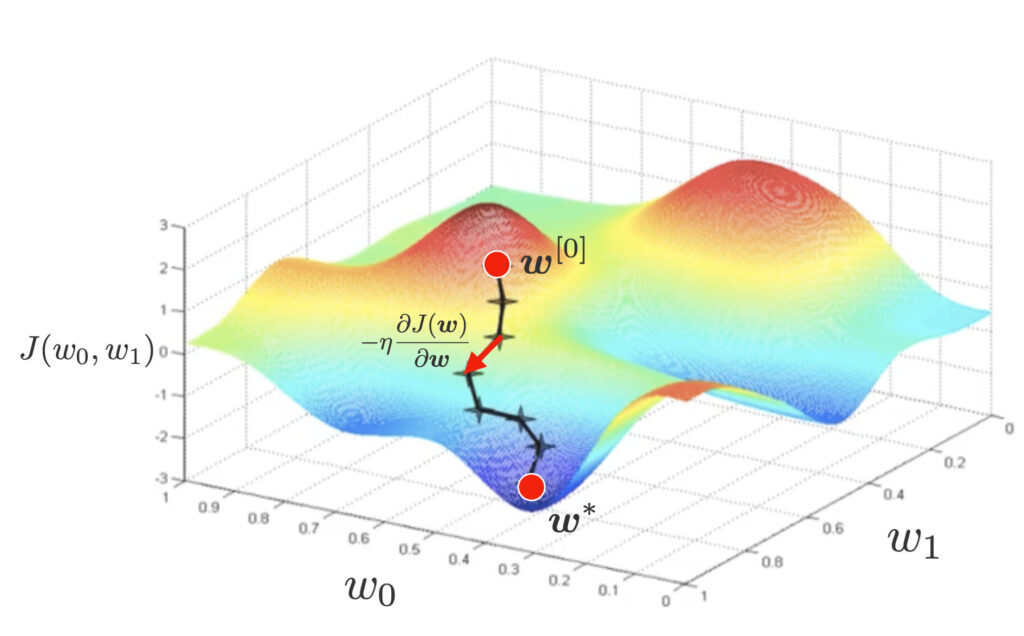
Now, since it is difficult to express the estimate $\bm{w}^*$ analytically in explicit form, we will use gradient descent to find the estimate. In gradient descent, we randomly set the initial value of the parameter $\bm{w}^{[0]}$ and update the parameter in the descent direction with a negative sign from the derivative as follows.
\bm{w}^{[t+1]} = \bm{w}^{[t]} – \eta\pd{J(\bm{w})}{\bm{w}}.
\end{align}
To perform gradient descent, let us calculate the value of the partial derivative $\pd{J(\bm{w})}{\bm{w}}$.
Calculation of Optimal Model Parameters
To calculate the value of the partial derivative $\pd{J(\bm{w})}{\bm{w}}$, we substitute $\eq{eq:proj}$ into $J(\bm{w})$ and simplify.
J(\bm{w}) &= \sum_{i=1}^n \[ -y^{(i)}\log p^{(i)} – (1-y^{(i)})\log (1 – p^{(i)}) \] \n
&\,\downarrow \textstyle\t \s{\text{Substitute }\eq{eq:proj}:\ p^{(i)} = \frac{1}{1+\exp(-\bm{w}^\T \bm{x}^{(i)})}} \n
&= \sum_{i=1}^n \biggl[-y^{(i)}\underbrace{\log \(\frac{1}{1+\exp(-\bm{w}^\T \bm{x}^{(i)})}\)}_{=\log1 – \log(1+\exp(-\bm{w}^\T \bm{x}^{(i)}))} – (1-y^{(i)})\underbrace{\log \(\frac{\exp(-\bm{w}^\T \bm{x}^{(i)})}{1+\exp(-\bm{w}^\T \bm{x}^{(i)})}\)}_{=-\bm{w}^\T\bm{x}^{(i)} – \log \(1 + \exp(-\bm{w}^\T \bm{x}^{(i)})\)} \biggr] \n
&= \sum_{i=1}^n \[y^{(i)}\log\(1+\exp(-\bm{w}^\T \bm{x}^{(i)})\) + (1-y^{(i)})\{\bm{w}^\T\bm{x}^{(i)} + \log \(1 + \exp(-\bm{w}^\T \bm{x}^{(i)})\) \} \] \n
&\,\downarrow \s{\text{Expand the second term}} \n
&= \sum_{i=1}^n \[ \cancel{y^{(i)}\log\(1+\exp(-\bm{w}^\T \bm{x}^{(i)})\)} + (1-y^{(i)})\bm{w}^\T\bm{x}^{(i)} + \log \(1 + \exp(-\bm{w}^\T \bm{x}^{(i)})\) \cancel{-y^{(i)}\log \(1 + \exp(-\bm{w}^\T \bm{x}^{(i)})\)} \] \n
&= \sum_{i=1}^n \underbrace{\[ (1-y^{(i)})\bm{w}^\T\bm{x}^{(i)} + \log \(1 + \exp(-\bm{w}^\T \bm{x}^{(i)})\) \]}_{=\varepsilon^{(i)}(\bm{w}) \text{ let this be}}.
\end{align*}
We want to take the partial derivative of the above expression with respect to $\bm{w}$, but since it is somewhat complicated, we will use the chain rule for composite functions. Let $u^{(i)} = \bm{w}^\T \bm{x}^{(i)}$ and decompose into the following expression.
\pd{J(\bm{w})}{\bm{w}} &= \pd{}{\bm{w}} \sum_{i=1}^n \varepsilon^{(i)}(\bm{w}) \n&= \sum_{i=1}^n \pd{\varepsilon^{(i)}(\bm{w})}{\bm{w}} \n&= \sum_{i=1}^n \pd{\varepsilon^{(i)}}{u^{(i)}} \pd{u^{(i)}}{\bm{w}}.\label{eq:chain}
\end{align}
1. Calculate the value of the partial derivative $\pd{\varepsilon^{(i)}}{u^{(i)}}$.
Now, since $\varepsilon^{(i)} = (1-y^{(i)})u^{(i)} + \log \(1 + \exp(-u^{(i)})\)$,
\pd{\varepsilon^{(i)}}{u^{(i)}} &= \pd{}{u^{(i)}} \[ (1-y^{(i)})u^{(i)} + \log \(1 + \exp(-u^{(i)})\) \] \n&= (1-y^{(i)}) – \f{\exp(-u^{(i)})}{1 + \exp(-u^{(i)})} \n&= \(1 – \f{\exp(-u^{(i)})}{1 + \exp(-u^{(i)})}\) – y^{(i)} \n&= \f{1}{1 + \exp(-u^{(i)})} – y^{(i)} \n&\,\downarrow \textstyle\t \s{\text{Substitute }\eq{eq:proj}:\ p^{(i)} = \frac{1}{1+\exp(-u^{(i)})}} \n&= p^{(i)} – y^{(i)}.\label{eq:pd_epsilon}
\end{align}
2. Calculate the value of the partial derivative $\pd{u^{(i)}}{\bm{w}}$.
\pd{u^{(i)}}{\bm{w}} &= \pd{(\bm{w}^\T \bm{x}^{(i)})}{\bm{w}} \n&= \bm{x}^{(i)}\ \ \because \s{\text{Formula for vector differentiation}}.\label{eq:pd_u}
\end{align}

From the above, by substituting $\eq{eq:pd_epsilon},(\ref{eq:pd_u})$ into $\eq{eq:chain}$
\pd{J(\bm{w})}{\bm{w}} = \sum_{i=1}^n \(p^{(i)} – y^{(i)} \) \bm{x}^{(i)}\label{eq:grad}
\end{align}
is obtained.
Matrix Notation for Optimal Model Parameters
As an alternative expression of $\eq{eq:grad}$, we show an expression using matrices.
We will express the observed $n$ pieces of $p$-dimensional data using matrices as follows.
\us X_{[n \times (p+1)]}=\mat{1 & x_1^{(1)} & x_2^{(1)} & \cdots & x_p^{(1)} \\ 1 & x_1^{(2)} & x_2^{(2)} &\cdots & x_p^{(2)} \\ \vdots & \vdots & \vdots & \ddots & \vdots \\ 1 & x_1^{(n)} & x_2^{(n)} &\cdots & x_p^{(n)}\\}.
\end{align*}
Also, we express the $n$ target variables $y^{(i)}$ and response probabilities $p^{(i)}$ using column vectors as follows.
\us \bm{y}_{[n \times 1]} = \mat{y^{(1)} \\ y^{(2)} \\ \vdots \\ y^{(n)}},\t\us \bm{p}_{[n\times 1]} = \mat{p^{(1)} \\ p^{(2)} \\ \vdots \\ p^{(n)}}.
\end{align*}
Using the above, let us write $\eq{eq:grad}$ in matrix notation.
\pd{J(\bm{w})}{\bm{w}} = \(\pd{J}{w_0},\pd{J}{w_1},\pd{J}{w_2}, \dots, \pd{J}{w_p} \)^\T
\end{align*}
Looking at the components of
\pd{J}{w_j} &= \sum_{i=1}^n \(p^{(i)} – y^{(i)} \) x^{(i)}_j \\&= \sum_{i=1}^n x^{(i)}_j \(p^{(i)} – y^{(i)} \) \\&(j = 0, 1, 2, \dots, p\t \s{where}\ x^{(i)}_0=1).
\end{align*}
Therefore, written in matrix form, it becomes the following expression.
\pd{J(\bm{w})}{\bm{w}} = \us \mat{\pd{J}{w_0} \\ \pd{J}{w_1} \\ \pd{J}{w_2} \\ \vdots \\ \pd{J}{w_p}}_{[(p+1) \times1]} = \underbrace{\us \mat{1 & 1 & \cdots & 1 \\ x^{(1)}_1 & x^{(2)}_1 & \cdots & x^{(n)}_1 \\ x^{(1)}_2 & x^{(2)}_2 & \cdots & x^{(n)}_2 \\ \vdots & \vdots & \ddots & \vdots \\ x^{(1)}_p & x^{(2)}_p & \cdots & x^{(n)}_p}_{[(p+1)\times n]}}_{=X^\T}\underbrace{\us \mat{p^{(1)} – y^{(1)} \\ p^{(2)} – y^{(2)} \\ \vdots \\ p^{(n)} – y^{(n)}}_{[n\times 1]}}_{=\bm{p}-\bm{y}}
\end{align*}
\therefore \pd{J(\bm{w})}{\bm{w}} =\large X^\T(\bm{p}\, -\, \bm{y}).
\end{align}
For the implementation of logistic regression, see here▼

の理解-〜実装編〜-120x68.jpg)